New Notes

Introduction to Solving Specific Equations

• In algebra, solving equations involves finding the values of variables that satisfy the given equation.
• This chapter focuses on solving equations of specific forms, including quadratic, rational, and equations involving roots or exponents.

---

General Strategies for Solving Equations

1. Identify the Type of Equation:
   • Recognize whether the equation is linear, quadratic, cubic, rational, or involves radicals or exponents.
2. Rearrange into Standard Form:
   • Rewrite the equation so that one side equals zero or isolate terms systematically.
3. Simplify the Equation:
   • Combine like terms, factorize expressions, or eliminate fractions or roots.
4. Solve Step-by-Step:
   • Use appropriate algebraic techniques depending on the equation type.
5. Verify Solutions:
   • Substitute solutions back into the original equation to ensure correctness.

---

Solving Quadratic Equations

• General form: ax2+bx+c=0ax^2 + bx + c = 0

1. Methods to Solve:
   • Factorization: (px+q)(rx+s)=0  ⟹  x=−qp,x=−sr(px + q)(rx + s) = 0 implies x = -frac{q}{p}, x = -frac{s}{r}
   • Completing the Square: ax2+bx+c=0  ⟹  a(x+b2a)2−b2−4ac4a=0ax^2 + bx + c = 0 implies aleft(x + frac{b}{2a}right)^2 – frac{b^2 – 4ac}{4a} = 0
   • Quadratic Formula: x=−b±b2−4ac2ax = frac{-b pm sqrt{b^2 – 4ac}}{2a}
   • Example: Solve 2×2−3x−2=02x^2 – 3x – 2 = 0:
     • Use the quadratic formula: x=−(−3)±(−3)2−4(2)(−2)2(2)x = frac{-(-3) pm sqrt{(-3)^2 – 4(2)(-2)}}{2(2)} x=3±9+164x = frac{3 pm sqrt{9 + 16}}{4} x=3±54x = frac{3 pm 5}{4} Solutions: x=2,x=−12x = 2, quad x = -frac{1}{2}

---

Solving Rational Equations

• Rational equations involve fractions with polynomials in the numerator and/or denominator.

1. Steps to Solve:
   • Identify and eliminate any restrictions on xx (values that make denominators zero).
   • Multiply through by the least common denominator (LCD) to eliminate fractions.
   • Solve the resulting equation (usually polynomial).
2. Example: Solve xx−2+3x+1=5×2−x−2frac{x}{x – 2} + frac{3}{x + 1} = frac{5}{x^2 – x – 2}:
   • Factor x2−x−2=(x−2)(x+1)x^2 – x – 2 = (x – 2)(x + 1), making the LCD (x−2)(x+1)(x – 2)(x + 1).
   • Multiply through by the LCD: x(x+1)+3(x−2)=5x(x + 1) + 3(x – 2) = 5
   • Simplify: x2+x+3x−6=5x^2 + x + 3x – 6 = 5 x2+4x−11=0x^2 + 4x – 11 = 0
   • Solve using the quadratic formula: x=−4±16+442x = frac{-4 pm sqrt{16 + 44}}{2} x=−4±602x = frac{-4 pm sqrt{60}}{2} x=−2±15x = -2 pm sqrt{15}

---

Solving Radical Equations

• Radical equations contain square roots or higher-order roots.

1. Steps to Solve:
   • Isolate the radical on one side of the equation.
   • Square both sides to eliminate the radical (or raise to the appropriate power).
   • Solve the resulting equation.
   • Check for extraneous solutions caused by squaring.
2. Example: Solve x+3=x−1sqrt{x + 3} = x – 1:
   • Square both sides: (x+3)2=(x−1)2(sqrt{x + 3})^2 = (x – 1)^2 x+3=x2−2x+1x + 3 = x^2 – 2x + 1
   • Rearrange: x2−3x−2=0x^2 – 3x – 2 = 0
   • Factorize: (x−2)(x+1)=0(x – 2)(x + 1) = 0
   • Solutions: x=2,x=−1x = 2, quad x = -1
   • Check:
     • For x=2x = 2: 2+3=2−1  ⟹  5=1(valid)sqrt{2 + 3} = 2 – 1 implies 5 = 1 quad (text{valid})
     • For x=−1x = -1: −1+3=−1−1(invalid, extraneous)sqrt{-1 + 3} = -1 – 1 quad (text{invalid, extraneous})

---

Solving Exponential Equations

• Exponential equations involve variables in exponents.

1. Steps to Solve:
   • Isolate the exponential term.
   • Apply logarithms to both sides.
   • Use logarithmic rules to solve for the variable.
2. Example: Solve 2x=162^x = 16:
   • Rewrite 1616 as a power of 2: 2x=242^x = 2^4
   • Equate exponents: x=4x = 4

---

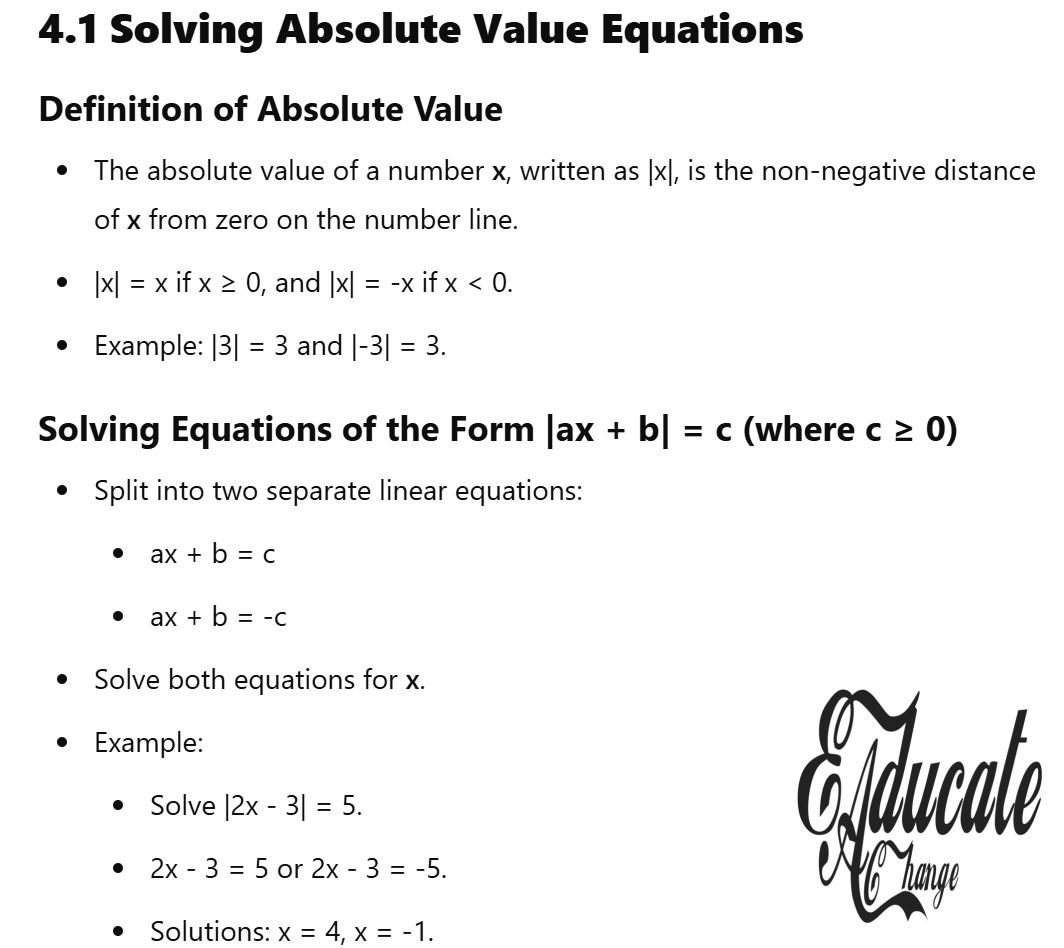
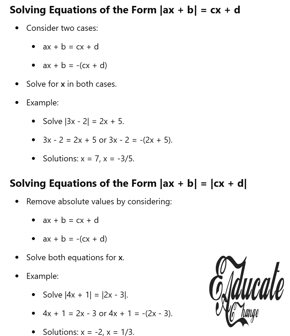
Solving Equations Involving Absolute Values

• Absolute value equations contain terms like ∣x∣|x|.

1. Steps to Solve:
   • Isolate the absolute value expression.
   • Rewrite the equation as two separate cases:
     1. x=+valuex = +text{value},
     2. x=−valuex = -text{value}.
2. Example: Solve ∣2x−3∣=5|2x – 3| = 5:
   • Case 1: 2x−3=52x – 3 = 5: 2x=8  ⟹  x=42x = 8 implies x = 4
   • Case 2: 2x−3=−52x – 3 = -5: 2x=−2  ⟹  x=−12x = -2 implies x = -1
   • Solutions: x=4,x=−1x = 4, quad x = -1

---

Applications of Equation Solving

1. Physics:
   • Modeling motion equations, force balances, and energy systems.
2. Engineering:
   • Structural analysis and system optimizations.
3. Economics:
   • Solving cost, profit, and demand-supply equations.

---

Practice Problems

1. Solve 3×2−5x+2=03x^2 – 5x + 2 = 0 using the quadratic formula.
2. Solve 2x−1+3x+1=5×2−1frac{2}{x – 1} + frac{3}{x + 1} = frac{5}{x^2 – 1}.
3. Solve 2x+5=x+1sqrt{2x + 5} = x + 1 and verify your solutions.
4. Solve 3x=813^x = 81 using logarithms.
5. Solve ∣x−4∣=7|x – 4| = 7 and find all possible values of xx.

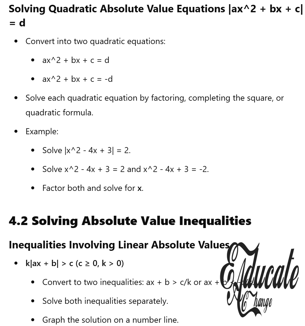
Introduction to Modulus Inequalities

• Modulus (or absolute value) inequalities involve expressions of the form ∣f(x)∣>c|f(x)| > c, ∣f(x)∣≥c|f(x)| geq c, ∣f(x)∣<c|f(x)| < c, or ∣f(x)∣≤c|f(x)| leq c, where c≥0c geq 0 is a constant.
• The modulus ∣f(x)∣|f(x)| represents the non-negative value of f(x)f(x), defined as: ∣f(x)∣={f(x),if f(x)≥0−f(x),if f(x)<0|f(x)| = begin{cases} f(x), & text{if } f(x) geq 0 \ -f(x), & text{if } f(x) < 0 end{cases}

---

Types of Modulus Inequalities

1. Strict Inequalities:
   • ∣f(x)∣>c|f(x)| > c or ∣f(x)∣<c|f(x)| < c.
   • These involve strict conditions where the modulus is either greater or less than a constant.
2. Inclusive Inequalities:
   • ∣f(x)∣≥c|f(x)| geq c or ∣f(x)∣≤c|f(x)| leq c.
   • These include the boundary cases where the modulus equals the constant.

---

General Approach to Solve Modulus Inequalities

1. Understand the Inequality:
   • Rewrite the inequality to consider the two possible cases for the modulus: positive and negative.
2. Split into Two Cases:
   • For ∣f(x)∣>c|f(x)| > c: f(x)>corf(x)<−cf(x) > c quad text{or} quad f(x) < -c
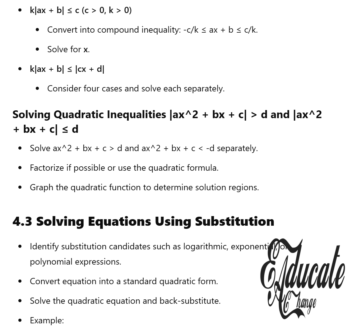
   • For ∣f(x)∣<c|f(x)| < c: −c<f(x)<c-c < f(x) < c
3. Solve Each Case Separately:
   • Solve the resulting inequalities step-by-step.
4. Combine Solutions:
   • Use the union or intersection of intervals to represent the solution, depending on the inequality type.
5. Graphical Interpretation:
   • Visualize the solution using a number line or graph, especially to check intersections.

---

Specific Cases of Modulus Inequalities

1. Case 1: ∣f(x)∣>c|f(x)| > c
   • The inequality ∣f(x)∣>c|f(x)| > c means the expression f(x)f(x) lies outside the interval [−c,c][-c, c].
   • Rewrite as two inequalities: f(x)>corf(x)<−cf(x) > c quad text{or} quad f(x) < -c
   • Example: Solve ∣2x−3∣>5|2x – 3| > 5:
     • Rewrite as: 2x−3>5or2x−3<−52x – 3 > 5 quad text{or} quad 2x – 3 < -5
     • Solve each inequality:
       • For 2x−3>52x – 3 > 5: 2x>8  ⟹  x>42x > 8 implies x > 4
       • For 2x−3<−52x – 3 < -5: 2x<−2  ⟹  x<−12x < -2 implies x < -1
     • Solution: x∈(−∞,−1)∪(4,∞)x in (-infty, -1) cup (4, infty)
2. Case 2: ∣f(x)∣≥c|f(x)| geq c
   • Similar to ∣f(x)∣>c|f(x)| > c, but includes the boundaries f(x)=cf(x) = c and f(x)=−cf(x) = -c.
   • Example: Solve ∣x+2∣≥3|x + 2| geq 3:
     • Rewrite as: x+2≥3orx+2≤−3x + 2 geq 3 quad text{or} quad x + 2 leq -3
     • Solve each inequality:
       • For x+2≥3x + 2 geq 3: x≥1x geq 1
       • For x+2≤−3x + 2 leq -3: x≤−5x leq -5
     • Solution: x∈(−∞,−5]∪[1,∞)x in (-infty, -5] cup [1, infty)
3. Case 3: ∣f(x)∣<c|f(x)| < c
   • The inequality ∣f(x)∣<c|f(x)| < c means f(x)f(x) lies strictly within the interval (−c,c)(-c, c).
   • Rewrite as: −c<f(x)<c-c < f(x) < c
   • Example: Solve ∣3x−4∣<7|3x – 4| < 7:
     • Rewrite as: −7<3x−4<7-7 < 3x – 4 < 7
     • Solve:
       • Add 4 to all sides: −3<3x<11-3 < 3x < 11
       • Divide by 3: −1<x<113-1 < x < frac{11}{3}
     • Solution: x∈(−1,113)x in (-1, frac{11}{3})
4. Case 4: ∣f(x)∣≤c|f(x)| leq c
   • Similar to ∣f(x)∣<c|f(x)| < c, but includes the boundaries f(x)=cf(x) = c and f(x)=−cf(x) = -c.
   • Example: Solve ∣x−5∣≤2|x – 5| leq 2:
     • Rewrite as: −2≤x−5≤2-2 leq x – 5 leq 2
     • Solve:
       • Add 5 to all sides: 3≤x≤73 leq x leq 7
     • Solution: x∈[3,7]x in [3, 7]

---

Graphical Representation of Modulus Inequalities

1. Visualizing on a Number Line:
   • Represent intervals for solutions on a number line to confirm union or intersection of ranges.
2. Using Graphs of y=∣f(x)∣y = |f(x)|:
   • Plot the modulus function y=∣f(x)∣y = |f(x)| and the constant y=cy = c.
   • Identify regions where ∣f(x)∣>c|f(x)| > c, ∣f(x)∣≥c|f(x)| geq c, ∣f(x)∣<c|f(x)| < c, or ∣f(x)∣≤c|f(x)| leq c.

---

Applications of Modulus Inequalities

1. Physics:
   • Used to model constraints in systems with non-negative quantities (e.g., magnitudes of forces).
2. Engineering:
   • Applied in designing systems with tolerances and thresholds.
3. Optimization:
   • Employed in finding feasible regions in constrained optimization problems.

---

Practice Problems

1. Solve ∣4x+3∣>7|4x + 3| > 7.
2. Solve ∣x−6∣≤4|x – 6| leq 4 and represent the solution graphically.
3. Solve ∣5x−1∣<8|5x – 1| < 8 and write the solution as an interval.
4. Solve ∣2x+1∣≥10|2x + 1| geq 10 and check the solution using a graph.

Introduction to Cubic Polynomials and Their Moduli

• Cubic polynomials are polynomials of degree three, expressed as: f(x)=ax3+bx2+cx+df(x) = ax^3 + bx^2 + cx + d where a≠0a neq 0, and a,b,c,da, b, c, d are constants.
• Modulus of a cubic polynomial:
  • Given f(x)f(x), the modulus function is ∣f(x)∣|f(x)|.
  • The modulus graph reflects the portions of the cubic graph that lie below the xx-axis upwards to lie above the xx-axis.

---

Characteristics of Cubic Polynomials

1. Degree and Shape:
   • The degree n=3n = 3 results in an S-shaped curve.
   • The graph may have up to two turning points.
2. Roots:
   • A cubic polynomial can have one, two, or three real roots.
   • The roots correspond to the xx-intercepts of the graph.
3. End Behavior:
   • As x→∞x to infty, f(x)→∞f(x) to infty if a>0a > 0, and f(x)→−∞f(x) to -infty if a<0a < 0.
   • As x→−∞x to -infty, f(x)→−∞f(x) to -infty if a>0a > 0, and f(x)→∞f(x) to infty if a<0a < 0.
4. Turning Points:
   • The graph can have up to two turning points where f′(x)=0f'(x) = 0.

---

Steps to Sketch a Cubic Polynomial

1. Identify Key Features:
   • Find the roots (solutions of f(x)=0f(x) = 0).
   • Determine the y-intercept (f(0)=df(0) = d).
   • Analyze the end behavior based on the sign of aa.
2. Calculate Turning Points:
   • Differentiate f(x)f(x) to get f′(x)f'(x), and solve f′(x)=0f'(x) = 0 to find critical points.
   • Determine whether each turning point is a local maximum, minimum, or inflection point by analyzing the second derivative f′′(x)f”(x).
3. Plot Key Points:
   • Mark the roots, y-intercept, and turning points on the graph.
   • Connect these points with a smooth curve, ensuring the graph aligns with the end behavior.
4. Check Symmetry (if applicable):
   • If b=0b = 0 and c=0c = 0, the cubic polynomial is symmetric about the origin (odd symmetry).

---

Example 1: Sketching a Cubic Polynomial

1. Given:f(x)=x3−3×2+2xf(x) = x^3 – 3x^2 + 2x
2. Find Roots:
   • Factorize: f(x)=x(x−1)(x−2)f(x) = x(x – 1)(x – 2)
     • Roots: x=0,1,2x = 0, 1, 2.
3. Determine End Behavior:
   • Since the leading coefficient a=1>0a = 1 > 0:
     • As x→∞x to infty, f(x)→∞f(x) to infty,
     • As x→−∞x to -infty, f(x)→−∞f(x) to -infty.
4. Find Turning Points:
   • Differentiate: f′(x)=3×2−6x+2f'(x) = 3x^2 – 6x + 2
     • Solve f′(x)=0f'(x) = 0: 3×2−6x+2=03x^2 – 6x + 2 = 0
       • Use the quadratic formula: x=−(−6)±(−6)2−4(3)(2)2(3)x = frac{-(-6) pm sqrt{(-6)^2 – 4(3)(2)}}{2(3)} x=6±126=6±236=1±33x = frac{6 pm sqrt{12}}{6} = frac{6 pm 2sqrt{3}}{6} = 1 pm frac{sqrt{3}}{3}
       • Turning points: x=1+33,x=1−33x = 1 + frac{sqrt{3}}{3}, x = 1 – frac{sqrt{3}}{3}.
5. Plot the Graph:
   • Roots at x=0,1,2x = 0, 1, 2,
   • Turning points at x=1±33x = 1 pm frac{sqrt{3}}{3},
   • End behavior guides the curve.

---

Sketching the Modulus of a Cubic Polynomial

1. Key Property of Modulus:
   • The modulus graph reflects the portions of the cubic graph below the xx-axis above the xx-axis.
   • For f(x)<0f(x) < 0, ∣f(x)∣=−f(x)|f(x)| = -f(x).
2. Steps to Sketch ∣f(x)∣|f(x)|:
   • Identify the intervals where f(x)≥0f(x) geq 0 and f(x)<0f(x) < 0.
   • Reflect the negative portions of the graph (where f(x)<0f(x) < 0) above the xx-axis.
3. Example:
   • Given f(x)=x3−3×2+2xf(x) = x^3 – 3x^2 + 2x:
     • Roots: x=0,1,2x = 0, 1, 2,
     • Negative intervals: 1<x<21 < x < 2.
     • Reflect the graph on 1<x<21 < x < 2 above the xx-axis to complete ∣f(x)∣|f(x)|.

---

Graphical Analysis of Modulus

1. Effect of Modulus on Roots:
   • The roots of f(x)=0f(x) = 0 remain unchanged in ∣f(x)∣=0|f(x)| = 0.
2. Turning Points:
   • Turning points below the xx-axis become local minima in the modulus graph.
3. Symmetry:
   • If f(x)f(x) is symmetric about the origin, ∣f(x)∣|f(x)| is symmetric about the y-axis.

---

Applications of Sketching Cubic Polynomials and Their Moduli

1. Physics:
   • Modeling displacement and force with cubic relationships.
2. Engineering:
   • Analyzing structural loads and stress variations.
3. Optimization:
   • Identifying ranges of positive and negative values in practical systems.

---

Practice Problems

1. Sketch f(x)=2×3−6×2+4xf(x) = 2x^3 – 6x^2 + 4x and its modulus.
2. Determine the turning points of f(x)=x3+3×2−9x−27f(x) = x^3 + 3x^2 – 9x – 27 and sketch ∣f(x)∣|f(x)|.
3. Analyze the behavior of f(x)=−x3+4×2−3xf(x) = -x^3 + 4x^2 – 3x and its modulus graphically.

Introduction to Cubic Inequalities

• Cubic inequalities involve expressions of the form f(x)>0f(x) > 0, f(x)<0f(x) < 0, f(x)≥0f(x) geq 0, or f(x)≤0f(x) leq 0, where f(x)f(x) is a cubic polynomial:f(x)=ax3+bx2+cx+df(x) = ax^3 + bx^2 + cx + dwhere a,b,c,da, b, c, d are constants, and a≠0a neq 0.
• The goal is to determine the range of xx-values where the inequality holds true by analyzing the graph of the cubic polynomial.

---

Key Concepts in Solving Cubic Inequalities

1. Roots of the Polynomial:
   • Roots of f(x)=0f(x) = 0 correspond to xx-intercepts of the graph.
2. Sign of the Polynomial:
   • The graph of f(x)f(x) divides the xx-axis into intervals where f(x)>0f(x) > 0 (above the xx-axis) and f(x)<0f(x) < 0 (below the xx-axis).
3. Nature of the Roots:
   • A cubic polynomial may have one, two, or three real roots.
   • Roots may be simple (crossing the xx-axis) or repeated (touching the xx-axis without crossing).
4. End Behavior:
   • The sign of the leading coefficient aa determines the graph’s behavior as x→∞x to infty and x→−∞x to -infty:
     • If a>0a > 0, the graph rises to ∞infty as x→∞x to infty and falls to −∞-infty as x→−∞x to -infty.
     • If a<0a < 0, the graph falls to −∞-infty as x→∞x to infty and rises to ∞infty as x→−∞x to -infty.

---

Steps to Solve Cubic Inequalities Graphically

1. Rewrite the Inequality:
   • Express the inequality in the form f(x)>0f(x) > 0, f(x)<0f(x) < 0, f(x)≥0f(x) geq 0, or f(x)≤0f(x) leq 0.
2. Find the Roots of f(x)=0f(x) = 0:
   • Solve f(x)=0f(x) = 0 to identify the xx-intercepts, using methods like factorization, synthetic division, or numerical approximation.
3. Determine the Sign of f(x)f(x) Between Roots:
   • Analyze the intervals between roots to determine where f(x)f(x) is positive or negative by testing points within each interval.
4. Sketch the Graph of f(x)f(x):
   • Plot the roots, turning points, and end behavior to sketch the graph accurately.
5. Interpret the Graph:
   • Use the graph to identify the intervals where the inequality holds true.

---

Solving Strict Inequalities (f(x)>0f(x) > 0 or f(x)<0f(x) < 0)

1. Strictly Greater Than (f(x)>0f(x) > 0):
   • Identify intervals where the graph lies above the xx-axis.
   • Exclude the points where f(x)=0f(x) = 0 (roots).
2. Strictly Less Than (f(x)<0f(x) < 0):
   • Identify intervals where the graph lies below the xx-axis.
   • Exclude the roots.

---

Solving Inclusive Inequalities (f(x)≥0f(x) geq 0 or f(x)≤0f(x) leq 0)

1. Greater Than or Equal To (f(x)≥0f(x) geq 0):
   • Include intervals where the graph lies above or touches the xx-axis.
   • Include the roots where f(x)=0f(x) = 0.
2. Less Than or Equal To (f(x)≤0f(x) leq 0):
   • Include intervals where the graph lies below or touches the xx-axis.
   • Include the roots where f(x)=0f(x) = 0.

---

Worked Examples

1. Example 1: Solving x3−6×2+11x−6>0x^3 – 6x^2 + 11x – 6 > 0
   • Step 1: Rewrite the inequality: f(x)=x3−6×2+11x−6>0f(x) = x^3 – 6x^2 + 11x – 6 > 0
   • Step 2: Find the roots:
     • Factorize: f(x)=(x−1)(x−2)(x−3)f(x) = (x – 1)(x – 2)(x – 3)
       • Roots: x=1,x=2,x=3x = 1, x = 2, x = 3.
   • Step 3: Analyze intervals:
     • Test points in each interval:
       • For x<1x < 1 (e.g., x=0x = 0): f(0)=(0−1)(0−2)(0−3)=(−1)(−2)(−3)=−6f(0) = (0 – 1)(0 – 2)(0 – 3) = (-1)(-2)(-3) = -6 f(x)<0f(x) < 0 for x<1x < 1.
       • For 1<x<21 < x < 2 (e.g., x=1.5x = 1.5): f(1.5)=(1.5−1)(1.5−2)(1.5−3)=(0.5)(−0.5)(−1.5)=0.375f(1.5) = (1.5 – 1)(1.5 – 2)(1.5 – 3) = (0.5)(-0.5)(-1.5) = 0.375 f(x)>0f(x) > 0 for 1<x<21 < x < 2.
       • For 2<x<32 < x < 3 (e.g., x=2.5x = 2.5): f(2.5)=(2.5−1)(2.5−2)(2.5−3)=(1.5)(0.5)(−0.5)=−0.375f(2.5) = (2.5 – 1)(2.5 – 2)(2.5 – 3) = (1.5)(0.5)(-0.5) = -0.375 f(x)<0f(x) < 0 for 2<x<32 < x < 3.
       • For x>3x > 3 (e.g., x=4x = 4): f(4)=(4−1)(4−2)(4−3)=(3)(2)(1)=6f(4) = (4 – 1)(4 – 2)(4 – 3) = (3)(2)(1) = 6 f(x)>0f(x) > 0 for x>3x > 3.
   • Step 4: Combine intervals: f(x)>0for x∈(1,2)∪(3,∞)f(x) > 0 quad text{for } x in (1, 2) cup (3, infty)
2. Example 2: Solving x3−4×2+6x−4≤0x^3 – 4x^2 + 6x – 4 leq 0
   • Step 1: Rewrite the inequality: f(x)=x3−4×2+6x−4≤0f(x) = x^3 – 4x^2 + 6x – 4 leq 0
   • Step 2: Find the roots:
     • Factorize: f(x)=(x−2)3f(x) = (x – 2)^3
       • Root: x=2x = 2 (triple root).
   • Step 3: Analyze the sign:
     • Since (x−2)3(x – 2)^3 changes sign only at x=2x = 2 and the polynomial has odd symmetry, the graph is non-positive (≤0leq 0) for all xx.
   • Step 4: Solution: f(x)≤0for x∈(−∞,2]f(x) leq 0 quad text{for } x in (-infty, 2]

---

Graphical Representation

1. Visualizing Solutions:
   • Plot f(x)f(x) on a graph and shade regions above (positive) or below (negative) the xx-axis depending on the inequality.
2. Turning Points and End Behavior:
   • Use the graph to identify key intervals for the solution.

---

Applications of Cubic Inequalities

1. Physics:
   • Used in modeling equilibrium points or constraints in systems.
2. Economics:
   • Solving profit or cost functions with cubic relationships.
3. Engineering:
   • Structural analysis for stress-strain relationships.

---

Practice Problems

1. Solve x3−3×2+2x>0x^3 – 3x^2 + 2x > 0 graphically.
2. Solve x3−2×2−x+2≤0x^3 – 2x^2 – x + 2 leq 0 and represent the solution graphically.
3. Analyze x3+6×2+11x+6>0x^3 + 6x^2 + 11x + 6 > 0 and sketch the graph.

Introduction to Complex Quadratic Equations

• Quadratic equations are of the general form: ax2+bx+c=0ax^2 + bx + c = 0 where a,b,ca, b, c are constants, and a≠0a neq 0.
• Complex quadratic equations refer to cases where:
  • The coefficients may include variables or additional expressions.
  • The equation requires advanced manipulation techniques to simplify and solve.

---

Characteristics of Quadratic Equations

1. Degree:
   • Quadratic equations are second-degree polynomials.
   • The highest power of the variable xx is 2.
2. Nature of Roots:
   • The roots of a quadratic equation can be real or complex, depending on the discriminant: Δ=b2−4acDelta = b^2 – 4ac
     • Δ>0Delta > 0: Two distinct real roots.
     • Δ=0Delta = 0: One repeated real root.
     • Δ<0Delta < 0: Two complex conjugate roots.

---

Strategies for Solving Complex Quadratic Equations

1. Rewriting into Standard Form:
   • Rearrange the equation so that all terms are on one side and it equals zero.
2. Simplify the Equation:
   • Combine like terms or simplify expressions to reduce the complexity.
3. Factorization:
   • If possible, factorize the quadratic expression into two linear factors: ax2+bx+c=(px+q)(rx+s)ax^2 + bx + c = (px + q)(rx + s)
   • Solve for xx by setting each factor equal to zero: px+q=0,rx+s=0px + q = 0, quad rx + s = 0
4. Quadratic Formula:
   • For non-factorable equations, use the quadratic formula: x=−b±b2−4ac2ax = frac{-b pm sqrt{b^2 – 4ac}}{2a}
5. Completing the Square:
   • Rewrite the quadratic equation in the form: a(x+b2a)2−b2−4ac4a2=0aleft(x + frac{b}{2a}right)^2 – frac{b^2 – 4ac}{4a^2} = 0
   • Solve for xx by isolating the squared term.

---

Types of Complex Quadratic Equations

1. Quadratic Equations with Fractions:
   • Fractions add complexity to the equation but can be simplified by multiplying through by the least common denominator (LCD).
   • Example: Solve:x23−x2=56frac{x^2}{3} – frac{x}{2} = frac{5}{6}
     • Multiply through by 6 (LCD): 6⋅x23−6⋅x2=6⋅566 cdot frac{x^2}{3} – 6 cdot frac{x}{2} = 6 cdot frac{5}{6} 2×2−3x=52x^2 – 3x = 5
     • Rearrange: 2×2−3x−5=02x^2 – 3x – 5 = 0
     • Solve using the quadratic formula: x=−(−3)±(−3)2−4(2)(−5)2(2)x = frac{-(-3) pm sqrt{(-3)^2 – 4(2)(-5)}}{2(2)} x=3±9+404x = frac{3 pm sqrt{9 + 40}}{4} x=3±494x = frac{3 pm sqrt{49}}{4} x=3±74x = frac{3 pm 7}{4} Roots: x=104=2.5,x=−44=−1x = frac{10}{4} = 2.5, quad x = frac{-4}{4} = -1
2. Quadratic Equations with Variables in the Denominator:
   • Equations where xx appears in the denominator require eliminating fractions.
   • Example: Solve:1x+2x+1=3frac{1}{x} + frac{2}{x+1} = 3
     • Multiply through by x(x+1)x(x + 1) (LCD): (x+1)+2x=3x(x+1)(x + 1) + 2x = 3x(x + 1) x+1+2x=3×2+3xx + 1 + 2x = 3x^2 + 3x
       • Rearrange: 3×2−2x−1=03x^2 – 2x – 1 = 0
       • Solve using the quadratic formula: x=−(−2)±(−2)2−4(3)(−1)2(3)x = frac{-(-2) pm sqrt{(-2)^2 – 4(3)(-1)}}{2(3)} x=2±4+126x = frac{2 pm sqrt{4 + 12}}{6} x=2±166x = frac{2 pm sqrt{16}}{6} x=2±46x = frac{2 pm 4}{6} Roots: x=1,x=−13x = 1, quad x = -frac{1}{3}
3. Quadratic Equations Involving Roots:
   • Equations containing square roots require isolating the root term and squaring both sides.
   • Example: Solve:x+3+x=5sqrt{x + 3} + x = 5
     • Isolate the square root: x+3=5−xsqrt{x + 3} = 5 – x
     • Square both sides: (x+3)2=(5−x)2(sqrt{x + 3})^2 = (5 – x)^2 x+3=25−10x+x2x + 3 = 25 – 10x + x^2
       • Rearrange: x2−11x+22=0x^2 – 11x + 22 = 0
       • Solve using the quadratic formula: x=−(−11)±(−11)2−4(1)(22)2(1)x = frac{-(-11) pm sqrt{(-11)^2 – 4(1)(22)}}{2(1)} x=11±121−882x = frac{11 pm sqrt{121 – 88}}{2} x=11±332x = frac{11 pm sqrt{33}}{2} Roots: x=11+332,x=11−332x = frac{11 + sqrt{33}}{2}, quad x = frac{11 – sqrt{33}}{2}
4. Quadratic Equations with Parameters:
   • Equations with unknown coefficients require solving for the parameter values.
   • Example: Solve x2+px+4=0x^2 + px + 4 = 0 such that the roots are equal:
     • Condition for equal roots: Δ=0Delta = 0 p2−4(1)(4)=0p^2 – 4(1)(4) = 0 p2−16=0p^2 – 16 = 0 p=±4p = pm 4

---

Applications of Solving Complex Quadratic Equations

1. Physics:
   • Modeling trajectories, wave motions, and force interactions.
2. Economics:
   • Finding profit and cost optimizations in economic models.
3. Engineering:
   • Solving structural and mechanical problems involving quadratic relationships.

---

Practice Problems

1. Solve 2×23−4×5=1frac{2x^2}{3} – frac{4x}{5} = 1.
2. Solve 1x+1+2x=3frac{1}{x+1} + frac{2}{x} = 3.
3. Solve x+4+2x=6sqrt{x + 4} + 2x = 6.
4. Find the parameter pp such that x2+px+9=0x^2 + px + 9 = 0 has one repeated root.