Straight Line Graphs (Copy)

New Notes

Introduction

Understanding the length of a line segment and its midpoint is foundational in geometry and forms the basis of coordinate geometry problems.
These calculations are critical for analyzing the properties of shapes and solving real-world problems in physics, engineering, and design.

Key Formulas

1. Length of a Line Segment

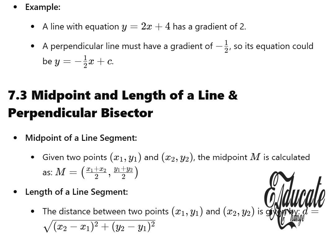
For two points $P(x1,y1)P(x_1, y_1)$ and $Q(x2,y2)Q(x_2, y_2)$ , the length $dd$ of the line segment $PQPQ$ is:

$d=(x2−x1)2+(y2−y1)2d = sqrt{(x_2 – x_1)^2 + (y_2 – y_1)^2}$

This formula is derived from the Pythagorean theorem.

2. Midpoint of a Line Segment

The midpoint $M(xm,ym)M(x_m, y_m)$ of the line segment joining $P(x1,y1)P(x_1, y_1)$ and $Q(x2,y2)Q(x_2, y_2)$ is:

$M=(x1+x22,y1+y22)M = left(frac{x_1 + x_2}{2}, frac{y_1 + y_2}{2}right)$

This gives the average of the x-coordinates and y-coordinates.

Applications

1. Distance Calculation

Used to determine the actual distance between two points in a coordinate system.
Common in navigation, construction, and 3D modeling.

2. Midpoint Usage

Helps locate the center of a segment, often used in symmetry, dividing line segments, and establishing geometric relationships.

Worked Examples

Example 1: Basic Distance and Midpoint

Find the length and midpoint of the line segment joining $A(-3,7)A(-3, 7)$ and $B(6,-2)B(6, -2)$ .

Length: $AB=(6−(−3))2+((−2)−7)2AB = sqrt{(6 – (-3))^2 + ((-2) – 7)^2}$ $AB=92+(−9)2=81+81=162≈12.73AB = sqrt{9^2 + (-9)^2} = sqrt{81 + 81} = sqrt{162} approx 12.73$
Midpoint: $M=(−3+62,7+(−2)2)M = left(frac{-3 + 6}{2}, frac{7 + (-2)}{2}right)$ $M=(32,52)=(1.5,2.5)M = left(frac{3}{2}, frac{5}{2}right) = (1.5, 2.5)$

Example 2: Finding Unknown Coordinates

The midpoint of the line segment joining $P(-5,11)P(-5, 11)$ and $Q(p,q)Q(p, q)$ is $M(2.5,-6)M(2.5, -6)$ . Find $pp$ and $qq$ .

Equations: $−5+p2=2.5and11+q2=−6frac{-5 + p}{2} = 2.5 quad text{and} quad frac{11 + q}{2} = -6$
Solve for $pp$ : $-5+p=5\Rightarrowp=10-5 + p = 5 quad Rightarrow quad p = 10$
Solve for $qq$ : $11+q=-12\Rightarrowq=-2311 + q = -12 quad Rightarrow quad q = -23$
Solution: $p=10, q=-23p = 10, , q = -23$

Example 3: Distance with Unknown Variables

The distance between $P(7,a)P(7, a)$ and $Q(a+1,9)Q(a+1, 9)$ is 15. Find $aa$ .

Equation: $(a+1−7)2+(9−a)2=15sqrt{(a + 1 – 7)^2 + (9 – a)^2} = 15$
Simplify: $(a−6)2+(9−a)2=15sqrt{(a – 6)^2 + (9 – a)^2} = 15$ $(a-6)2+(9-a)2=225(a - 6)^2 + (9 - a)^2 = 225$ Expand: $a2-12a+36+81-18a+a2=225a^2 - 12a + 36 + 81 - 18a + a^2 = 225$ Combine:
$2a2-30a+117=2252a^2 - 30a + 117 = 225$ Simplify further:

$a2-15a-54=0a^2 - 15a - 54 = 0$ Factorize:

$(a-18)(a+3)=0(a - 18)(a + 3) = 0$
Solutions: $a=18ora=-3a = 18 quad text{or} quad a = -3$

Example 4: Finding Coordinates in a Parallelogram

Three vertices of a parallelogram are $A(-10,1)A(-10, 1)$ , $B(6,-2)B(6, -2)$ , and $C(14,4)C(14, 4)$ . Find the fourth vertex $DD$ .

Midpoint of $ACAC$ : $M=(−10+142,1+42)=(2,2.5)M = left(frac{-10 + 14}{2}, frac{1 + 4}{2}right) = (2, 2.5)$
Equating midpoints: The midpoint of $BDBD$ must also be $M(2,2.5)M(2, 2.5)$ .
Coordinates of $DD$ : Let $D(m,n)D(m, n)$ . Solve: $6+m2=2⇒m=−2frac{6 + m}{2} = 2 quad Rightarrow quad m = -2$ $−2+n2=2.5⇒n=7frac{-2 + n}{2} = 2.5 quad Rightarrow quad n = 7$
Solution: $D=(-2,7)D = (-2, 7)$

Additional Practice Problems

Find the length of the line joining:
- $P(2,0)P(2, 0)$ and $Q(5,0)Q(5, 0)$ .
- $P(-7,4)P(-7, 4)$ and $Q(-7,8)Q(-7, 8)$ .
Find the coordinates of the midpoint for:
- $A(4,3)A(4, 3)$ and $B(9,11)B(9, 11)$ .
- $P(-1,7)P(-1, 7)$ and $Q(2,-4)Q(2, -4)$ .
A point $P(2k,k)P(2k, k)$ is equidistant from $A(-2,4)A(-2, 4)$ and $B(7,-5)B(7, -5)$ . Find $kk$ .

Summary

The length and midpoint formulas are essential tools in coordinate geometry.
They allow us to compute distances, locate midpoints, and solve problems involving unknown coordinates.
These concepts have applications in geometry, physics, and practical design challenges.

Key Concepts and Definitions

1. Gradient (Slope)

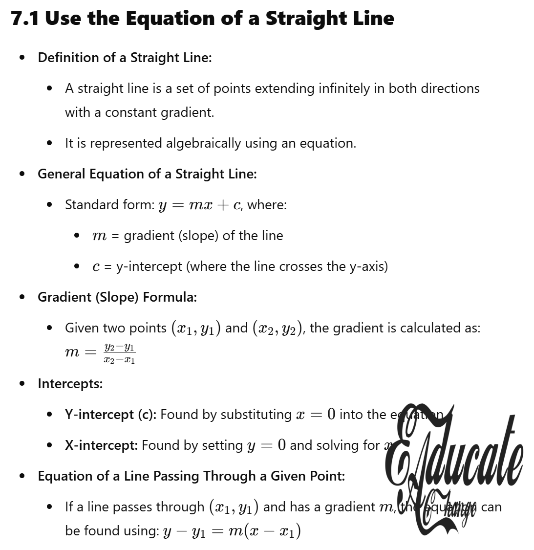
The gradient $mm$ of a straight line measures its steepness and is calculated as: $m=y2−y1x2−x1m = frac{y_2 – y_1}{x_2 – x_1}$ for two points $(x1,y1)(x_1, y_1)$ and $(x2,y2)(x_2, y_2)$ on the line.

2. Parallel Lines

Definition: Lines are parallel if they have the same gradient but different y-intercepts.
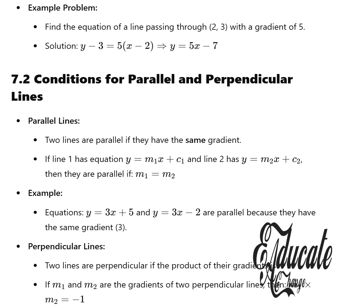
- For two lines with gradients $m1m_1$ and $m2m_2$ , if $m1=m2m_1 = m_2$ , the lines are parallel.
Equation: Parallel lines take the form $y=mx+c1y = mx + c_1$ and $y=mx+c2y = mx + c_2$ , where $c1\neqc2c_1 neq c_2$ .

3. Perpendicular Lines

Definition: Two lines are perpendicular if the product of their gradients is −1-1.
- If $m1m_1$ is the gradient of one line and $m2m_2$ is the gradient of the other, then: $m1\cdotm2=-1m_1 cdot m_2 = -1$
Reciprocal Rule: The gradient of one line is the negative reciprocal of the other.

Equations of Straight Lines

1. General Form

The equation of a straight line is: y=mx+cy = mx + c where:
- $mm$ is the gradient.
- $cc$ is the y-intercept (the point where the line crosses the y-axis).

2. Point-Slope Form

If a line passes through a known point $(x1,y1)(x_1, y_1)$ with gradient $mm$ , its equation is: $y-y1=m(x-x1)y - y_1 = m(x - x_1)$

3. Horizontal and Vertical Lines

Horizontal lines have a gradient $m=0m = 0$ and equation $y=cy = c$ .
Vertical lines have an undefined gradient and equation $x=ax = a$ , where $aa$ is a constant.

Worked Examples

Example 1: Gradient of Parallel Lines

Find the gradient of a line parallel to $y=3x+4y = 3x + 4$ .

Solution:
- The gradient of the given line is $m=3m = 3$ .
- A parallel line will also have $m=3m = 3$ .
- Example parallel equation: $y=3x-2y = 3x - 2$ .

Example 2: Perpendicular Lines

Find the gradient of a line perpendicular to $y=12x−5y = frac{1}{2}x – 5$ .

Solution:
- Gradient of the given line: $m1=12m_1 = frac{1}{2}$ .
- Perpendicular gradient $m2m_2$ satisfies: $m1⋅m2=−1⇒12⋅m2=−1m_1 cdot m_2 = -1 quad Rightarrow quad frac{1}{2} cdot m_2 = -1$ $m2=-2m_2 = -2$
- Example perpendicular equation: $y=-2x+3y = -2x + 3$ .

Example 3: Checking Collinearity

Determine if points $A(2,3)A(2, 3)$ , $B(4,7)B(4, 7)$ , and $C(6,11)C(6, 11)$ are collinear.

Solution:
1. Find the gradient of $ABAB$ : $mAB=7−34−2=2m_{AB} = frac{7 – 3}{4 – 2} = 2$
2. Find the gradient of $BCBC$ : $mBC=11−76−4=2m_{BC} = frac{11 – 7}{6 – 4} = 2$
3. Since $mAB=mBCm_{AB} = m_{BC}$ , the points are collinear.

Example 4: Equation of a Perpendicular Bisector

Find the equation of the perpendicular bisector of the line joining $A(3,2)A(3, 2)$ and $B(7,10)B(7, 10)$ .

Solution:
1. Midpoint: $M=(3+72,2+102)=(5,6)M = left(frac{3 + 7}{2}, frac{2 + 10}{2}right) = (5, 6)$
2. Gradient of $ABAB$ : $mAB=10−27−3=2m_{AB} = frac{10 – 2}{7 – 3} = 2$
3. Perpendicular Gradient: $mperpendicular=−12m_{text{perpendicular}} = -frac{1}{2}$
4. Equation: $y−6=−12(x−5)y – 6 = -frac{1}{2}(x – 5)$ $y=−12x+52+6y = -frac{1}{2}x + frac{5}{2} + 6$ $y=−12x+172y = -frac{1}{2}x + frac{17}{2}$

Applications

1. Geometric Problems

Collinearity: Checking if points lie on the same line by comparing gradients.
Perpendicular Bisectors: Useful in constructing medians, altitudes, and circumcenters in geometry.

2. Real-World Contexts

Road and rail alignments often use parallel and perpendicular lines for intersection design.
Engineering projects, such as bridges, use perpendicular bisectors for structural integrity.

Practice Problems

Find the equation of the line parallel to $y=4x-3y = 4x - 3$ and passing through $(2,5)(2, 5)$ .
Find the equation of the line perpendicular to $y=−34x+2y = -frac{3}{4}x + 2$ and passing through $(0,-1)(0, -1)$ .
Determine if the points $(1,2)(1, 2)$ , $(3,6)(3, 6)$ , and $(5,10)(5, 10)$ are collinear.
Find the equation of the perpendicular bisector of the line segment joining $(2,-3)(2, -3)$ and $(-4,7)(-4, 7)$ .

Summary

Parallel lines share the same gradient, while perpendicular lines have gradients that multiply to $-1-1$ .
Equations of lines can be formulated in various forms depending on the information provided.
Applications span geometry, navigation, and structural engineering. The concepts of parallel and perpendicular lines are essential for solving both theoretical and applied problems.

Key Concepts and Formulas

1. Definition of a Straight Line

The equation of a straight line can be written in the general form: y=mx+cy = mx + c where:
- $mm$ : Gradient (slope) of the line.
- $cc$ : y-intercept (the value of $yy$ when $x=0x = 0$ ).

2. Gradient

Gradient $mm$ is calculated as: $m=y2−y1x2−x1m = frac{y_2 – y_1}{x_2 – x_1}$ for two points $(x1,y1)(x_1, y_1)$ and $(x2,y2)(x_2, y_2)$ .

3. Point-Slope Form

If a line passes through a point $(x1,y1)(x_1, y_1)$ and has a gradient $mm$ , its equation is: $y-y1=m(x-x1)y - y_1 = m(x - x_1)$

4. Intercept Form

In cases where both x-intercept ( $aa$ ) and y-intercept ( $bb$ ) are known: $xa+yb=1frac{x}{a} + frac{y}{b} = 1$

5. Horizontal and Vertical Lines

Horizontal lines: $y=k(gradient m=0).y = k quad text{(gradient ( m = 0 ))}.$
Vertical lines: $x=h(gradient undefined).x = h quad text{(gradient undefined)}.$

Key Techniques and Applications

1. Finding the Equation of a Line

Given a gradient and a point:

Example:

Gradient ( m = 2 ), point ( (4, 7) ):
Equation:
y - 7 = 2(x - 4) quad Rightarrow quad y = 2x - 1

Given two points (x1,y1)(x_1, y_1) and (x2,y2)(x_2, y_2):
1. Find the gradient: $m=y2−y1x2−x1m = frac{y_2 – y_1}{x_2 – x_1}$
2. Use the point-slope form.

2. Finding Parallel and Perpendicular Lines

Parallel Lines:
- Have the same gradient ( $m1=m2m_1 = m_2$ ).
- Example:
```
Line: ( y = 3x + 2 ).
Parallel line: ( y = 3x - 4 ).
```
Perpendicular Lines:
- Gradients satisfy $m1\cdotm2=-1m_1 cdot m_2 = -1$ .
- Example:
```
Line: ( y = 2x + 1 ).
Perpendicular line: ( y = -frac{1}{2}x + c ).
```

3. Midpoint and Length

Midpoint: $M=(x1+x22,y1+y22)M = left(frac{x_1 + x_2}{2}, frac{y_1 + y_2}{2}right)$
Length of a Line Segment: $d=(x2−x1)2+(y2−y1)2d = sqrt{(x_2 – x_1)^2 + (y_2 – y_1)^2}$

4. Special Applications

Collinearity:
- Points are collinear if the gradients between each pair are equal.
Intersection of Lines:
- Solve simultaneous equations for two line equations.

Worked Examples

Example 1: Find the Equation of a Line

Find the equation of the line passing through $(3,2)(3, 2)$ and $(7,6)(7, 6)$ .

Step 1: Calculate gradient: $m=6−27−3=1m = frac{6 – 2}{7 – 3} = 1$
Step 2: Use point-slope form: $y-2=1(x-3)\Rightarrowy=x-1y - 2 = 1(x - 3) quad Rightarrow quad y = x - 1$

Example 2: Perpendicular Bisector

Find the equation of the perpendicular bisector of the line joining $(4,6)(4, 6)$ and $(8,10)(8, 10)$ .

Step 1: Find midpoint: $M=(4+82,6+102)=(6,8)M = left(frac{4 + 8}{2}, frac{6 + 10}{2}right) = (6, 8)$
Step 2: Find gradient of the line: $m=10−68−4=1m = frac{10 – 6}{8 – 4} = 1$
Step 3: Gradient of perpendicular line: $mperpendicular=−1m_{text{perpendicular}} = -1$
Step 4: Equation of perpendicular bisector: $y-8=-1(x-6)\Rightarrowy=-x+14y - 8 = -1(x - 6) quad Rightarrow quad y = -x + 14$

Example 3: Intersection of Lines

Find the intersection of $y=2x-3y = 2x - 3$ and $y=-x+5y = -x + 5$ .

Step 1: Solve simultaneous equations: $2x-3=-x+52x - 3 = -x + 5$ $3x=8⇒x=833x = 8 quad Rightarrow quad x = frac{8}{3}$
Step 2: Substitute $xx$ into one equation: $y=2(83)−3=163−3=73y = 2left(frac{8}{3}right) – 3 = frac{16}{3} – 3 = frac{7}{3}$
Solution: $(83,73)left(frac{8}{3}, frac{7}{3}right)$

Practice Problems

Find the equation of the line passing through $(2,5)(2, 5)$ and parallel to $y=3x-7y = 3x - 7$ .
Determine if the points $(1,2)(1, 2)$ , $(3,6)(3, 6)$ , and $(5,10)(5, 10)$ are collinear.
Find the point of intersection for $y=12x+1y = frac{1}{2}x + 1$ and $y=-2x+4y = -2x + 4$ .
Write the equation of a line perpendicular to $y=−34x+2y = -frac{3}{4}x + 2$ passing through $(0,-1)(0, -1)$ .

Summary

This chapter covers the foundational aspects of straight-line equations:

Gradient, intercepts, and the forms of equations.
Techniques to find parallel and perpendicular lines.
Special applications like midpoint, collinearity, and intersections.

Introduction

The area of rectilinear figures, such as triangles, quadrilaterals, and polygons, is calculated using various geometric and algebraic methods.
Two common approaches:
1. Coordinate Geometry Method: Employs vertices coordinates.
2. Shoestring/Shoelace Method: A systematic formula for calculating polygon areas using coordinates.

General Formula for Area of a Triangle

Definition:
- For vertices $A(x1,y1)A(x_1, y_1)$ , $B(x2,y2)B(x_2, y_2)$ , and $C(x3,y3)C(x_3, y_3)$ , the area $AA$ of the triangle is given by: $A=12∣x1y2+x2y3+x3y1−y1x2−y2x3−y3x1∣A = frac{1}{2} left| x_1y_2 + x_2y_3 + x_3y_1 – y_1x_2 – y_2x_3 – y_3x_1 right|$
- Note: The absolute value ensures the area is non-negative.
Steps to Calculate:
- Multiply x-coordinates by the next y-coordinate in sequence.
- Multiply y-coordinates by the next x-coordinate in sequence.
- Subtract the sum of the second set of products from the first.
- Divide by 2.
Example:
- Given $A(1,3)A(1, 3)$ , $B(9,1)B(9, 1)$ , and $C(3,8)C(3, 8)$ : $A=12∣(1⋅1)+(9⋅8)+(3⋅3)−(3⋅9)−(1⋅3)−(8⋅1)∣A = frac{1}{2} left| (1 cdot 1) + (9 cdot 8) + (3 cdot 3) – (3 cdot 9) – (1 cdot 3) – (8 cdot 1) right|$ $A=12∣1+72+9−27−3−8∣=12∣44∣=22A = frac{1}{2} left| 1 + 72 + 9 – 27 – 3 – 8 right| = frac{1}{2} left| 44 right| = 22$

Shoelace Method

Definition:
- A simplified approach to calculate the area of polygons (triangles, quadrilaterals, or more complex shapes).
Procedure:
- List coordinates of vertices sequentially, repeating the first point at the end.
- Multiply each x-coordinate by the next y-coordinate in sequence.
- Multiply each y-coordinate by the next x-coordinate in sequence.
- Take the absolute difference of sums and divide by 2.
Example for a Pentagon:
- Given vertices $A(0,-1)A(0, -1)$ , $B(5,1)B(5, 1)$ , $C(3,4)C(3, 4)$ , $D(-1,6)D(-1, 6)$ , $E(-3,2)E(-3, 2)$ : $A=12∣0⋅1+5⋅4+3⋅6+(−1)⋅2+(−3)⋅(−1)−(−1⋅5)−(1⋅3)−(4⋅(−1))−(6⋅(−3))−(2⋅0)∣A = frac{1}{2} left| 0 cdot 1 + 5 cdot 4 + 3 cdot 6 + (-1) cdot 2 + (-3) cdot (-1) – (-1 cdot 5) – (1 cdot 3) – (4 cdot (-1)) – (6 cdot (-3)) – (2 cdot 0) right|$ $A=12∣0+20+18−2+3−(−5)−3−(−4)−(−18)−0∣=12∣42∣=31.5A = frac{1}{2} left| 0 + 20 + 18 – 2 + 3 – (-5) – 3 – (-4) – (-18) – 0 right| = frac{1}{2} left| 42 right| = 31.5$

Area of Quadrilaterals

Split into Triangles:
- Divide the quadrilateral into two triangles by drawing a diagonal.
- Calculate the area of each triangle using the triangle area formula and sum them.
Coordinate Geometry Formula:
- Generalized formula: $A=12∣x1y2+x2y3+x3y4+x4y1−(y1x2+y2x3+y3x4+y4x1)∣A = frac{1}{2} left| x_1y_2 + x_2y_3 + x_3y_4 + x_4y_1 – (y_1x_2 + y_2x_3 + y_3x_4 + y_4x_1) right|$
Example:
- For $A(1,8)A(1, 8)$ , $B(-4,5)B(-4, 5)$ , $C(-2,-3)C(-2, -3)$ , $D(4,-2)D(4, -2)$ : $A=12∣1⋅5+(−4)⋅(−3)+(−2)⋅(−2)+4⋅8−(8⋅−4+5⋅−2+−3⋅4+−2⋅1)∣A = frac{1}{2} left| 1 cdot 5 + (-4) cdot (-3) + (-2) cdot (-2) + 4 cdot 8 – (8 cdot -4 + 5 cdot -2 + -3 cdot 4 + -2 cdot 1) right|$ $A=12∣5+12+4+32−(−32−10−12−2)∣=12∣53∣=26.5A = frac{1}{2} left| 5 + 12 + 4 + 32 – (-32 – 10 – 12 – 2) right| = frac{1}{2} left| 53 right| = 26.5$

Alternative Methods

1. Boxing-In Method

Enclose the polygon in a rectangle or square.
Subtract the areas of the external triangles or rectangles.

2. Grid Method

Use a grid to approximate the area by counting squares within the polygon.

Applications

Engineering:
- Structural design calculations often require precise polygon area measurements.
Physics:
- Areas represent quantities like work done or fields in diagrams.
Land Surveying:
- Determining land areas for mapping or property boundaries.

Worked Problems

Find the Area of Triangle $ABCABC$ :
- $A(-2,3)A(-2, 3)$ , $B(0,-4)B(0, -4)$ , $C(5,6)C(5, 6)$ : $A=12∣−2(−4)+0(6)+5(3)−3(0)−(−4)(5)−6(−2)∣A = frac{1}{2} left| -2(-4) + 0(6) + 5(3) – 3(0) – (-4)(5) – 6(-2) right|$ $A=12∣8+0+15−0−(−20)−(−12)∣=28.5A = frac{1}{2} left| 8 + 0 + 15 – 0 – (-20) – (-12) right| = 28.5$
Find the Area of Quadrilateral $PQRSPQRS$ :
- $P(2,7)P(2, 7)$ , $Q(-5,6)Q(-5, 6)$ , $R(-3,-4)R(-3, -4)$ , $S(7,2)S(7, 2)$ : $A=12∣2⋅6+(−5)⋅(−4)+(−3)⋅2+7⋅7−(7⋅−5+6⋅−3+−4⋅7+2⋅2)∣A = frac{1}{2} left| 2 cdot 6 + (-5) cdot (-4) + (-3) cdot 2 + 7 cdot 7 – (7 cdot -5 + 6 cdot -3 + -4 cdot 7 + 2 cdot 2) right|$ Solve systematically.

Key Tips

Sequence of Vertices:
- Always list vertices in a consistent order (clockwise or counterclockwise) to avoid sign errors.
Coordinate Accuracy:
- Ensure precise vertex coordinates for accurate area calculations.
Units:
- Area values should always be expressed with the correct units.

Introduction

Non-Linear to Linear Conversion:
- Many real-world phenomena are modeled by non-linear equations.
- Converting these into linear form simplifies analysis, especially using graphs and regression methods.
Straight Line Representation:
- The standard linear form is: Y=mX+cY = mX + c where:
  - $mm$ is the gradient (slope).
  - $cc$ is the y-intercept.

Steps for Conversion

Identify the Non-Linear Equation:
- Begin with an equation involving variables $xx$ and $yy$ .
- Example: $y=axby = ax^b$ , $y=aebxy = ae^{bx}$ , or $y=ax+by = frac{a}{x} + b$ .
Choose Suitable Variables:
- Replace the original variables with expressions that transform the equation into a straight line.
- Example:
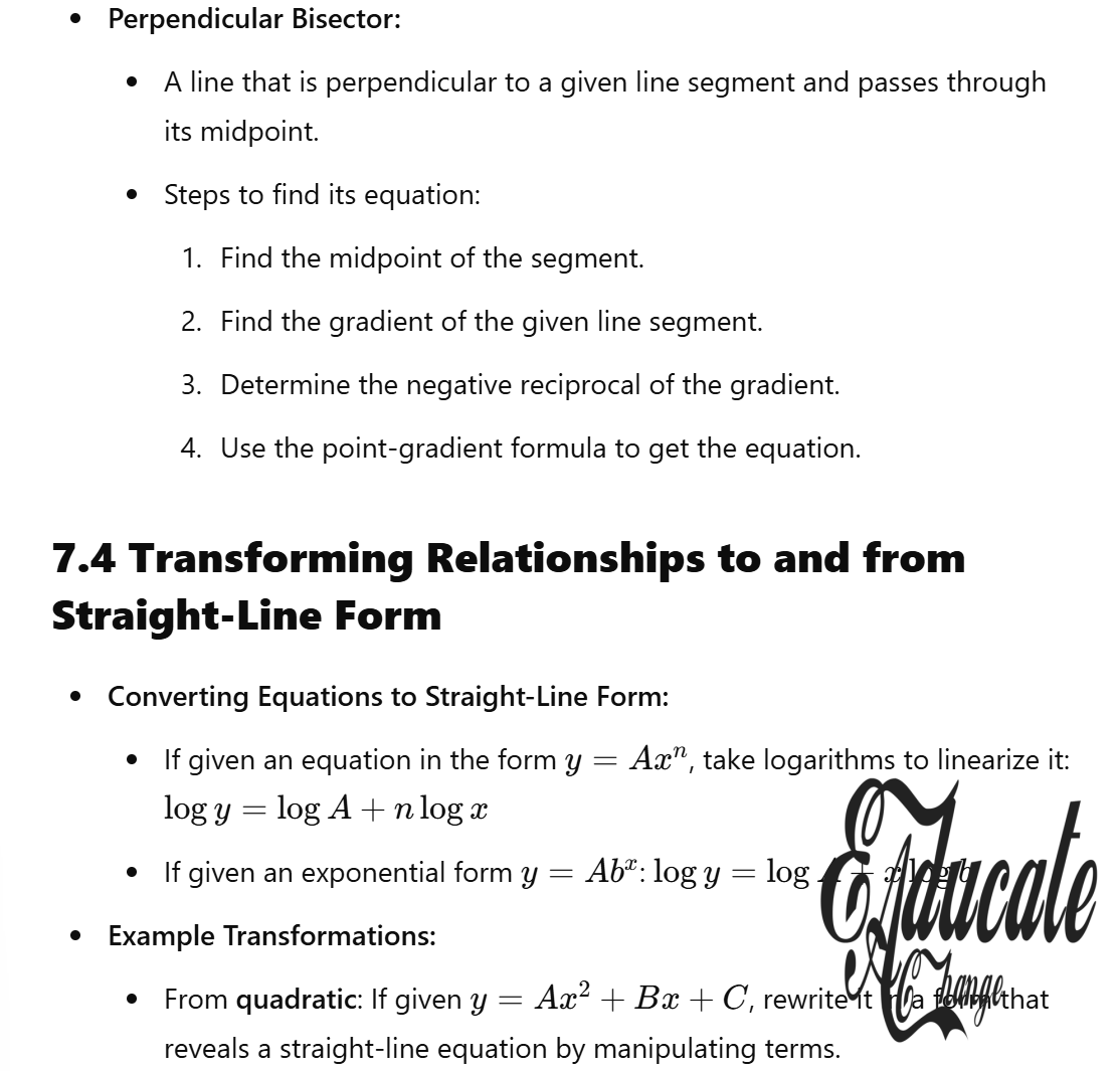
  - For y=axby = ax^b, take logarithms on both sides to get: log⁡y=blog⁡x+log⁡alog y = b log x + log a
    - Here, $Y=logyY = log y$ , $X=logxX = log x$ , $m=bm = b$ , and $c=logac = log a$ .
Reformulate Using Logarithmic or Other Transformations:
- Apply transformations to isolate a linear relationship.
- Example:
  - For y=aebxy = ae^{bx}, take the natural logarithm: ln⁡y=bx+ln⁡aln y = bx + ln a
    - Here, $Y=lnyY = ln y$ , $X=xX = x$ , $m=bm = b$ , and $c=lnac = ln a$ .
Plot the Transformed Variables:
- Plot the new variables $YY$ and $XX$ to form a straight-line graph.
- The gradient and intercept of the graph give the constants of the original equation.

Worked Examples

Example 1: Exponential Equation

Convert $y=aebxy = ae^{bx}$ into linear form.

Solution:
- Take natural logarithms: ln⁡y=bx+ln⁡aln y = bx + ln a
  - $Y=lnyY = ln y$ , $X=xX = x$ , $m=bm = b$ , $c=lnac = ln a$ .
- The transformed equation is: $Y=mX+cY = mX + c$

Example 2: Power Law

Convert $y=axby = ax^b$ into linear form.

Solution:
- Take logarithms on both sides: log⁡y=blog⁡x+log⁡alog y = b log x + log a
  - $Y=logyY = log y$ , $X=logxX = log x$ , $m=bm = b$ , $c=logac = log a$ .

Key Points to Note

Variable Definitions:
- The newly defined variables $YY$ and $XX$ should represent only the original variables $xx$ and $yy$ .
- Constants $mm$ and $cc$ should depend solely on the original parameters.
Interpretation:
- The gradient $mm$ from the linear graph corresponds to specific constants (e.g., exponent or coefficient).
- The y-intercept $cc$ provides additional parameters of the original equation.
Alternative Methods:
- Multiplication or division by $xx$ or other transformations can sometimes simplify the equation further.

Worked Example 3: Practical Scenario

Given $y=ax+by = frac{a}{x} + b$ , convert to linear form.

Solution:
- Multiply through by $xx$ : $yx=a+bxyx = a + bx$
- Rearrange: $y=ax+b⇒Y=y,X=1x,m=b,c=a.y = frac{a}{x} + b quad Rightarrow quad Y = y, X = frac{1}{x}, m = b, c = a.$

Worked Example 4: Logarithmic Data

Variables $xx$ and $yy$ satisfy $y=axby = ax^b$ . Plot data and find $aa$ and $bb$ .

Steps:
- Take logarithms: log⁡y=blog⁡x+log⁡alog y = b log x + log a
  - Plot $logylog y$ (Y) against $logxlog x$ (X).
- Gradient $b=slope of the lineb = text{slope of the line}$ .
- Intercept $loga=clog a = c$ .

Graphical Interpretations

Gradient and Intercept:
- The slope of the straight line represents the exponent or proportional constant.
- The intercept represents an additive or multiplicative constant.
Applications:
- Use graphing techniques to estimate constants $aa$ and $bb$ in equations.

Applications in Real Life

Physics:
- Analyze exponential decay or growth phenomena, such as radioactive decay or capacitor discharge.
Economics:
- Model growth trends using power laws.
Engineering:
- Fit experimental data to models using logarithmic or exponential relationships.

Practice Problems

Convert $y=5\times2+3y = 5x^2 + 3$ into linear form.
For $y=aebxy = ae^{bx}$ , identify $aa$ and $bb$ using data points.
Given $y=2x+5y = frac{2}{x} + 5$ , plot and find the constants using linear graphs.

Key Concept

Reverse Transformation:
- Conversion of a linear equation $Y=mX+cY = mX + c$ into its original non-linear form is a reverse process of linearization.
- Used to derive original equations from experimental data or graphing relationships.

Key Steps

Understand the Linear Equation:
- Start with the given linear form: $Y=mX+cY = mX + c$ where $YY$ and $XX$ are transformed variables representing original variables $yy$ and $xx$ .
Substitute Back into the Non-Linear Form:
- Replace $YY$ and $XX$ with their definitions in terms of $xx$ and $yy$ .
Simplify the Expression:
- Rearrange to express $yy$ in terms of $xx$ and the original constants.

Worked Examples

Example 1: Exponential Growth

Given $Y=-bX+lnaY = -bX + ln a$ , convert to the non-linear equation.

Substitute Definitions:
- $Y=lnyY = ln y$ , $X=xX = x$ .
Reformulate: $lny=-bx+lnaln y = -bx + ln a$
Exponentiate Both Sides: $y=eln⁡a−bx=ae−bxy = e^{ln a – bx} = ae^{-bx}$
Result: The non-linear equation is $y=ae−bxy = ae^{-bx}$ .

Example 2: Power Law

Given $Y=mX+cY = mX + c$ , where $Y=logyY = log y$ and $X=logxX = log x$ , convert to the non-linear form.

Substitute Definitions: $logy=mlogx+clog y = m log x + c$
Simplify Using Logarithmic Properties: $logy=log(xm)+logklog y = log(x^m) + log k$ where $k=10ck = 10^c$ .
Combine Logs: $logy=log(kxm)log y = log(kx^m)$
Exponentiate Both Sides: $y=kxmy = kx^m$

Gradient and Intercept Interpretation

Gradient ( $mm$ ):
- Represents a parameter in the non-linear equation (e.g., $bb$ in $y=aebxy = ae^{bx}$ or $mm$ in $y=kxmy = kx^m$ ).
Intercept ( $cc$ ):
- Often relates to a multiplicative constant (e.g., $lnaln a$ or $logklog k$ ).

Graphical Approach

Plot the Linearized Data:
- Example: $Y=lnyY = ln y$ vs. $X=xX = x$ produces a straight line.
Determine Slope and Intercept:
- Gradient gives the exponent or proportional factor.
- Intercept determines the constant in the non-linear form.

Key Observations

Ensure that $XX$ and $YY$ are appropriately defined in terms of $xx$ and $yy$ .
The original constants must be recovered explicitly, requiring careful substitution and rearrangement.

Applications

Experimental Data Analysis:
- Reverse linearization helps model real-world phenomena like population growth, radioactive decay, or economic trends.
Physics and Engineering:
- Recovers underlying equations from simplified data representations.

Practice Problems

Given: Y=3X+2Y = 3X + 2, Y=ln⁡yY = ln y, and X=ln⁡xX = ln x.
- Find the non-linear equation.
- Answer: $y=e2x3y = e^2x^3$ .
Given: Y=−2X+5Y = -2X + 5, Y=ln⁡yY = ln y, X=xX = x.
- Find the non-linear equation.
- Answer: $y=e5e−2xy = e^5e^{-2x}$ .
Given: Y=4X−1Y = 4X – 1, Y=yY = y, X=x2X = x^2.
- Find the non-linear equation.
- Answer: $y=4\times2-1y = 4x^2 - 1$ .

Summary

Converting linear forms back into non-linear equations is a vital skill for interpreting experimental relationships and mathematical modeling.
Each transformation depends on the definitions of $YY$ and $XX$ , requiring a step-by-step approach to ensure accuracy.
Applications span scientific, engineering, and mathematical disciplines.

Introduction

Experimental data often shows relationships between two variables, $xx$ and $yy$ .
The goal is to find a mathematical model connecting these variables, which can often be linear or non-linear.
Non-linear relationships can be converted to a straight-line form for simplicity using logarithmic or other transformations.

Key Concepts

1. Identifying a Relationship

Straight-Line Relationship:
- If the data forms a straight line when graphed, it follows the general form: y=mx+cy = mx + c where:
  - $mm$ is the gradient (slope).
  - $cc$ is the y-intercept.
Curved Relationship:
- More commonly, data forms a curve, connected by a non-linear equation like:
  - $y=kxny = kx^n$
  - $y=aebxy = ae^{bx}$

2. Linearizing Non-Linear Equations

Transforming non-linear equations into linear form involves:
1. Applying logarithms or other operations to simplify the equation.
2. Re-defining variables to match the linear form $Y=mX+cY = mX + c$ .

3. Graphing and Interpreting Results

The transformed equation is plotted as a straight line.
Gradient and intercept values are used to extract constants of the original relationship.

Worked Examples

Example 1: Power Law

Given experimental data, show that $yy$ and $xx$ are related by $y=kxny = kx^n$ .

Non-Linear Equation: $y=kxny = kx^n$
Take Logarithms: $logy=logk+nlogxlog y = log k + n log x$
Linear Form:Y=nX+CY = nX + Cwhere:
- $Y=logyY = log y$
- $X=logxX = log x$
- $C=logkC = log k$ .
Procedure:
- Plot $logylog y$ against $logxlog x$ .
- Gradient $n=ΔYΔXn = frac{Delta Y}{Delta X}$ .
- Intercept $C=logkC = log k$ , so $k=10Ck = 10^C$ .

Example 2: Exponential Relationship

Given $y=aebxy = ae^{bx}$ , show the relationship between $yy$ and $xx$ .

Non-Linear Equation: $y=aebxy = ae^{bx}$
Take Natural Logarithm: $lny=bx+lnaln y = bx + ln a$
Linear Form:Y=mX+CY = mX + Cwhere:
- $Y=lnyY = ln y$
- $X=xX = x$
- $m=bm = b$
- $C=lnaC = ln a$ .
Procedure:
- Plot $lnyln y$ against $xx$ .
- Gradient $m=bm = b$ .
- Intercept $C=lnaC = ln a$ , so $a=eCa = e^C$ .

Steps to Solve

Transform the Equation:
- Use logarithmic or algebraic transformations to convert a non-linear equation into linear form.
Create a Data Table:
- Add columns for the transformed variables $XX$ and $YY$ .
Plot the Data:
- Use the transformed variables for graphing.
Analyze the Graph:
- Determine the gradient and intercept.
Reconstruct the Original Equation:
- Substitute the gradient and intercept values back to find the constants of the original equation.

Worked Example: Logarithmic Relationship

Problem:

Variables $xx$ and $yy$ are related as $y=axby = ax^b$ .
Data points: $(x,y)=(10,1596),(20,983),(40,605),(80,372)(x, y) = (10, 1596), (20, 983), (40, 605), (80, 372)$ .

Solution:

Transform the Equation:log⁡y=blog⁡x+log⁡alog y = b log x + log a
- $Y=logyY = log y$
- $X=logxX = log x$
- $C=logaC = log a$ .
Compute Values:
- Add $logylog y$ and $logxlog x$ columns to the data table.
Plot $logylog y$ vs. $logxlog x$ :
- Gradient $bb$ : Calculate using two points: $b=ΔYΔXb = frac{Delta Y}{Delta X}$
- Intercept $CC$ : Use $logy=blogx+logalog y = b log x + log a$ to find $logalog a$ .
Reconstruct the Equation:
- $a=10log⁡aa = 10^{log a}$ .
- Final equation: $y=axby = ax^b$ .

Applications

Physics:
- Analyze relationships like Hooke’s Law or radioactive decay.
Economics:
- Fit growth models, such as exponential growth of investments.
Engineering:
- Model material properties, such as stress-strain curves.

Practice Problems

Experimental data suggests y∝xny propto x^n. Transform and find nn and kk for:
- $x={1,2,3,4},y={10,40,90,160}x = {1, 2, 3, 4}, y = {10, 40, 90, 160}$ .
Show that $y=aebxy = ae^{bx}$ holds for $x={1,2,3,4},y={3,5.5,10,18}x = {1, 2, 3, 4}, y = {3, 5.5, 10, 18}$ .
The table below shows experimental values for yy and xx. Derive the constants aa and bb for y=axby = ax^b:
- $x={10,20,40,80},y={1596,983,605,372}x = {10, 20, 40, 80}, y = {1596, 983, 605, 372}$ .

Conclusion

Finding relationships from data combines mathematical transformations, plotting, and analytical skills.
Transformations like logarithms simplify complex relationships, enabling a deeper understanding of variable dependencies.
Applications range from experimental physics to predictive modeling in diverse fields.

EAC

Education

Support

Other Projects

Want To Teach Online?