New Notes

Introduction to Further Vector Notation

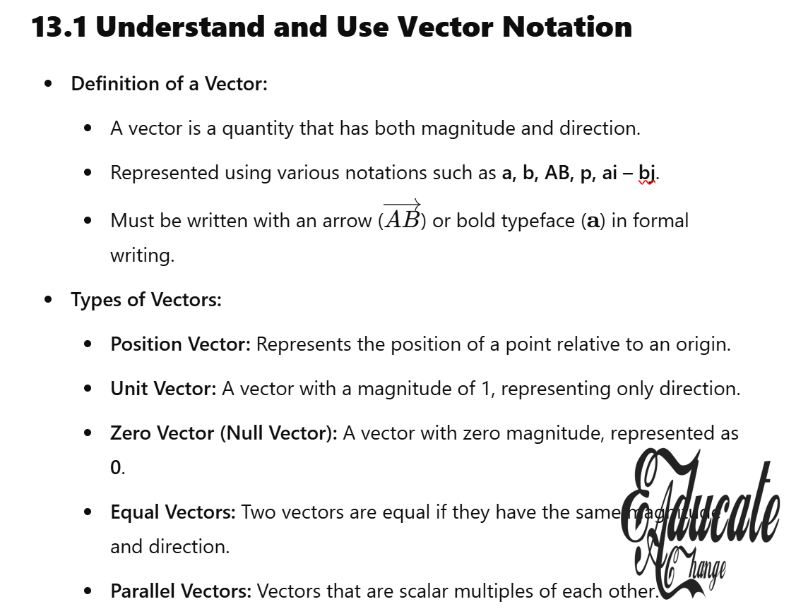
• Vectors are quantities that have both magnitude and direction.
• The notation and methods used to represent and work with vectors are crucial for solving geometry and physics problems involving displacement, velocity, and forces.
• This chapter builds on basic vector knowledge, introducing more advanced concepts of vector representation and manipulation.

Vector Representation

1. Component Form:
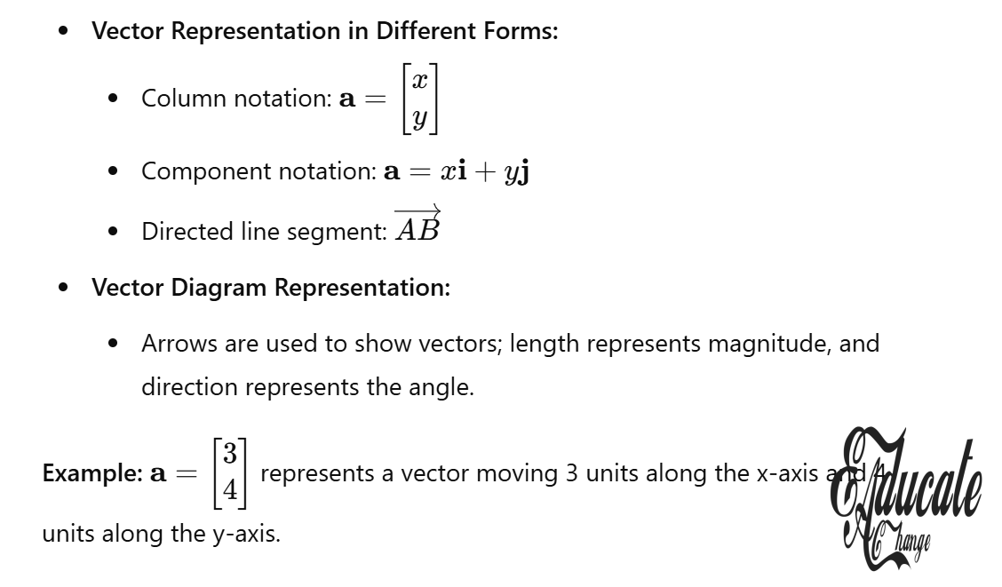
   • A vector in 2-dimensional space can be written in component form as: v=ai+bjmathbf{v} = ai + bj where aa is the x-component and bb is the y-component of the vector.
     • Unit vectors:
       • imathbf{i} represents the unit vector in the direction of the x-axis.
       • jmathbf{j} represents the unit vector in the direction of the y-axis.
     • Example:
       • A vector ABmathbf{AB} from point A(4,7)A(4, 7) to B(3,4)B(3, 4) can be written as: AB=(3−4)i+(4−7)j=−i−3jmathbf{AB} = (3-4) mathbf{i} + (4-7) mathbf{j} = -mathbf{i} – 3mathbf{j}
2. Magnitude of a Vector:
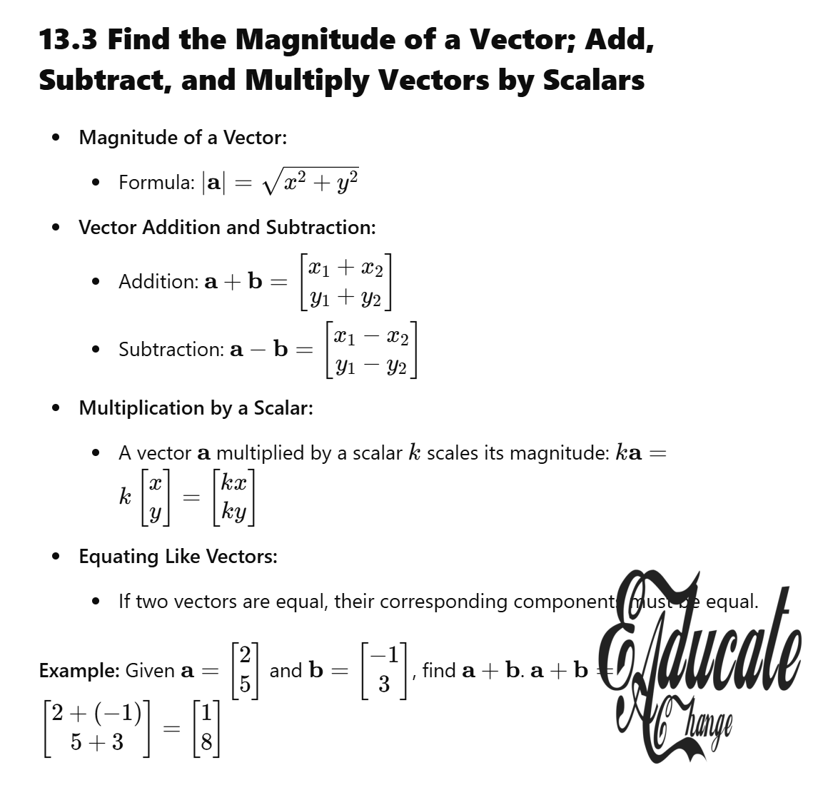
   • The magnitude (or modulus) of a vector v=ai+bjmathbf{v} = ai + bj is calculated using the Pythagorean theorem: ∣v∣=a2+b2|mathbf{v}| = sqrt{a^2 + b^2}
     • Example:
       • For the vector v=4i+3jmathbf{v} = 4mathbf{i} + 3mathbf{j}, the magnitude is: ∣v∣=42+32=16+9=25=5|mathbf{v}| = sqrt{4^2 + 3^2} = sqrt{16 + 9} = sqrt{25} = 5
3. Unit Vector:
   • A unit vector is a vector with a magnitude of 1.
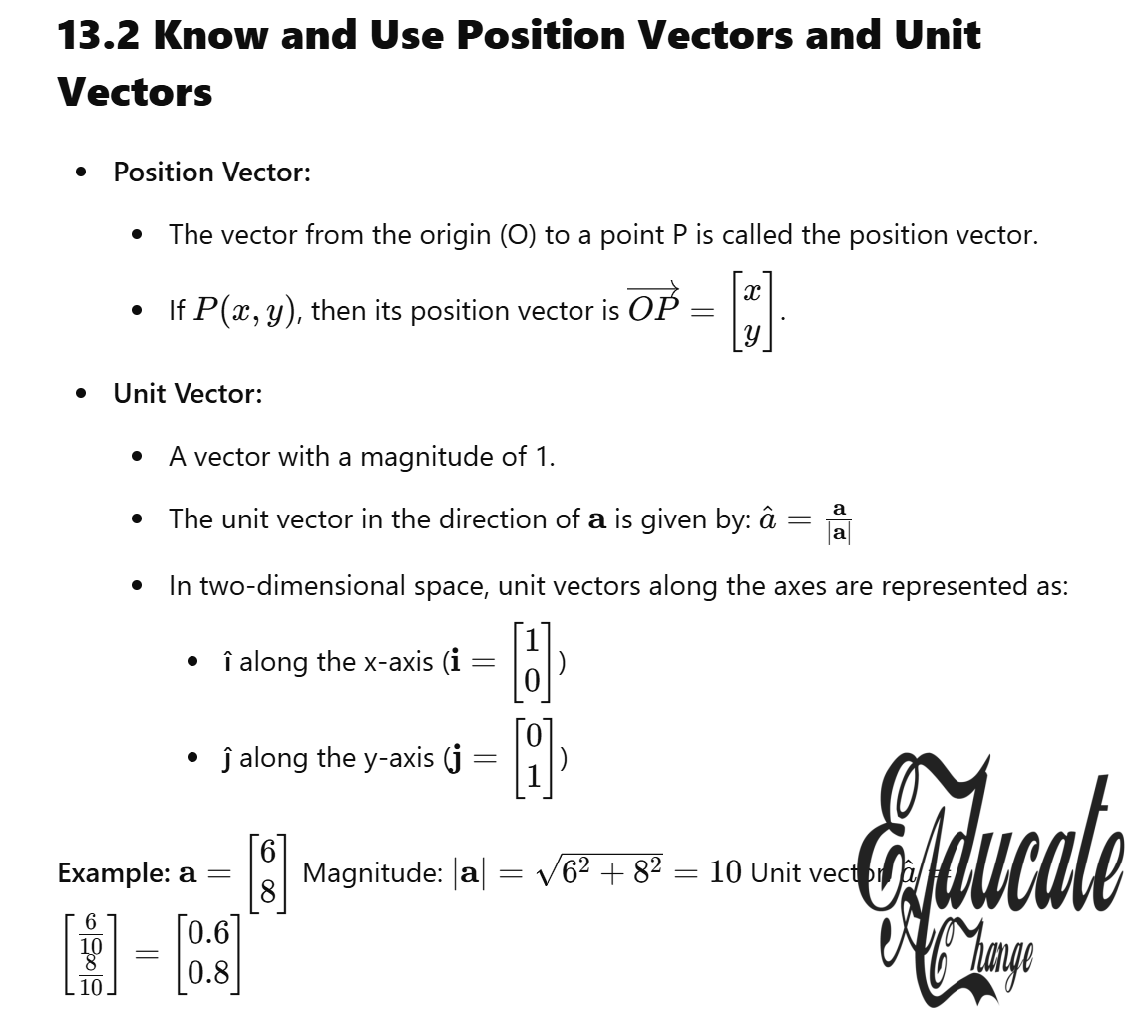
   • The unit vector in the direction of a given vector v=ai+bjmathbf{v} = ai + bj is: v^=1∣v∣vhat{v} = frac{1}{|mathbf{v}|} mathbf{v}
     • Example:
       • For v=4i+3jmathbf{v} = 4mathbf{i} + 3mathbf{j}, the unit vector is: v^=15(4i+3j)=45i+35jhat{v} = frac{1}{5} (4mathbf{i} + 3mathbf{j}) = frac{4}{5} mathbf{i} + frac{3}{5} mathbf{j}

Addition and Subtraction of Vectors

1. Vector Addition:
   • Vectors are added component-wise. If u=ai+bjmathbf{u} = ai + bj and v=ci+djmathbf{v} = ci + dj, their sum is: u+v=(a+c)i+(b+d)jmathbf{u} + mathbf{v} = (a + c)mathbf{i} + (b + d)mathbf{j}
     • Example:
       • If u=4i+3jmathbf{u} = 4mathbf{i} + 3mathbf{j} and v=−2i+5jmathbf{v} = -2mathbf{i} + 5mathbf{j}, then: u+v=(4−2)i+(3+5)j=2i+8jmathbf{u} + mathbf{v} = (4 – 2)mathbf{i} + (3 + 5)mathbf{j} = 2mathbf{i} + 8mathbf{j}
2. Vector Subtraction:
   • Vector subtraction is also done component-wise. If u=ai+bjmathbf{u} = ai + bj and v=ci+djmathbf{v} = ci + dj, their difference is: u−v=(a−c)i+(b−d)jmathbf{u} – mathbf{v} = (a – c)mathbf{i} + (b – d)mathbf{j}
     • Example:
       • If u=4i+3jmathbf{u} = 4mathbf{i} + 3mathbf{j} and v=−2i+5jmathbf{v} = -2mathbf{i} + 5mathbf{j}, then: u−v=(4+2)i+(3−5)j=6i−2jmathbf{u} – mathbf{v} = (4 + 2)mathbf{i} + (3 – 5)mathbf{j} = 6mathbf{i} – 2mathbf{j}

Multiplying Vectors by Scalars

• A vector can be multiplied by a scalar (a number), which scales the vector’s magnitude but keeps its direction.
• If v=ai+bjmathbf{v} = ai + bj and kk is a scalar, the result of multiplying the vector by kk is: kv=(ka)i+(kb)jkmathbf{v} = (ka)mathbf{i} + (kb)mathbf{j}
  • Example:
    • If v=4i+3jmathbf{v} = 4mathbf{i} + 3mathbf{j} and k=2k = 2, then: kv=2(4i+3j)=8i+6jkmathbf{v} = 2(4mathbf{i} + 3mathbf{j}) = 8mathbf{i} + 6mathbf{j}

Parallel Vectors

• Two vectors are parallel if they have the same direction or if one is a scalar multiple of the other.
• If u=ai+bjmathbf{u} = ai + bj and v=ci+djmathbf{v} = ci + dj, then umathbf{u} and vmathbf{v} are parallel if: ac=bdfrac{a}{c} = frac{b}{d}
  • Example:
    • If u=4i+3jmathbf{u} = 4mathbf{i} + 3mathbf{j} and v=8i+6jmathbf{v} = 8mathbf{i} + 6mathbf{j}, they are parallel because: 48=36=12frac{4}{8} = frac{3}{6} = frac{1}{2}

Work with Position Vectors

1. Position Vector:
   • The position vector of a point PP relative to an origin OO is the vector that points from OO to PP.
   • If point PP has coordinates (x,y)(x, y), then the position vector of PP is written as: OP=xi+yjmathbf{OP} = xmathbf{i} + ymathbf{j}
   • Example:
     • The position vector of point P(4,7)P(4, 7) relative to the origin is: OP=4i+7jmathbf{OP} = 4mathbf{i} + 7mathbf{j}
2. Displacement Vector:
   • The displacement vector from point AA with position vector amathbf{a} to point BB with position vector bmathbf{b} is: AB=b−amathbf{AB} = mathbf{b} – mathbf{a}
   • Example:
     • If AA has position vector a=2i+3jmathbf{a} = 2mathbf{i} + 3mathbf{j} and BB has position vector b=5i+7jmathbf{b} = 5mathbf{i} + 7mathbf{j}, then the displacement vector is: AB=(5i+7j)−(2i+3j)=3i+4jmathbf{AB} = (5mathbf{i} + 7mathbf{j}) – (2mathbf{i} + 3mathbf{j}) = 3mathbf{i} + 4mathbf{j}

Vector Geometry Problems

1. Midpoint of a Line Segment:
   • The midpoint of a line segment connecting points AA and BB with position vectors amathbf{a} and bmathbf{b} is given by: M=a+b2mathbf{M} = frac{mathbf{a} + mathbf{b}}{2}
   • Example:
     • If AA has position vector a=2i+3jmathbf{a} = 2mathbf{i} + 3mathbf{j} and BB has position vector b=5i+7jmathbf{b} = 5mathbf{i} + 7mathbf{j}, then the midpoint MM is: M=(2i+3j)+(5i+7j)2=7i+10j2=3.5i+5jmathbf{M} = frac{(2mathbf{i} + 3mathbf{j}) + (5mathbf{i} + 7mathbf{j})}{2} = frac{7mathbf{i} + 10mathbf{j}}{2} = 3.5mathbf{i} + 5mathbf{j}
2. Collinearity of Vectors:
   • Points are said to be collinear if the vectors representing the points are parallel.
   • Example:
     • If AA, BB, and CC are points on a line, then the vectors ABmathbf{AB} and BCmathbf{BC} must be parallel.

---

Practice Problems

1. Write each vector in the form ai+bjai + bj.
   • a) ABmathbf{AB}, ACmathbf{AC}, AEmathbf{AE}
   • b) BEmathbf{BE}, AFmathbf{AF}, CEmathbf{CE}
2. Find the magnitude of the following vectors:
   • a) −2i-2mathbf{i}
   • b) 4i+3j4mathbf{i} + 3mathbf{j}
3. Find the unit vector in the direction of the following vectors:
   • a) 6i+8j6mathbf{i} + 8mathbf{j}
   • b) −4i−3j-4mathbf{i} – 3mathbf{j}

---

Summary

• Vector Notation is essential for describing quantities in physics and geometry, as vectors represent both magnitude and direction.
• Component form, magnitude, and unit vectors provide the foundation for solving problems.
• Addition, subtraction, and scalar multiplication are core operations that are crucial for manipulating vectors.
• Position vectors and displacement vectors help describe movement and spatial relationships between points.

Introduction to Position Vectors

1. Definition of Position Vector:
   • A position vector represents the location of a point in space relative to a chosen origin.
   • If OO is the origin and P(x,y,z)P(x, y, z) is a point in three-dimensional space, the position vector OPmathbf{OP} is denoted by: OP=⟨x,y,z⟩mathbf{OP} = langle x, y, z rangle
     • Where ⟨x,y,z⟩langle x, y, z rangle are the coordinates of the point PP in the Cartesian coordinate system.
   • In two-dimensional space, the position vector is written as: OP=⟨x,y⟩mathbf{OP} = langle x, y rangle
     • Here, the vector gives the displacement from the origin O(0,0)O(0, 0) to the point P(x,y)P(x, y).

---

Representation of Vectors

2. Vector Notation:
   • Vectors are typically represented as boldface letters or with an arrow above, such as: v,a,bmathbf{v}, mathbf{a}, mathbf{b} or OP→,AB→overrightarrow{OP}, overrightarrow{AB}
   • Vectors can be represented by their components in a coordinate system. In 2D or 3D space, a vector vmathbf{v} can be written as:
     • In 2D: v=⟨vx,vy⟩mathbf{v} = langle v_x, v_y rangle
     • In 3D: v=⟨vx,vy,vz⟩mathbf{v} = langle v_x, v_y, v_z rangle
3. Direction of Position Vectors:
   • The position vector describes not only the magnitude (or length) of the displacement but also the direction from the origin to the point.
   • The magnitude of the position vector OPmathbf{OP}, denoted by ∣OP∣|mathbf{OP}|, is given by: ∣OP∣=x2+y2+z2|mathbf{OP}| = sqrt{x^2 + y^2 + z^2} for 3D space. For 2D, this becomes: ∣OP∣=x2+y2|mathbf{OP}| = sqrt{x^2 + y^2}

---

Calculating Position Vectors

4. Position Vector Between Two Points:
   • Given two points A(x1,y1,z1)A(x_1, y_1, z_1) and B(x2,y2,z2)B(x_2, y_2, z_2), the position vector from AA to BB is the vector that starts at AA and ends at BB. This is calculated by subtracting the coordinates of AA from those of BB: AB→=⟨x2−x1,y2−y1,z2−z1⟩overrightarrow{AB} = langle x_2 – x_1, y_2 – y_1, z_2 – z_1 rangle In 2D: AB→=⟨x2−x1,y2−y1⟩overrightarrow{AB} = langle x_2 – x_1, y_2 – y_1 rangle
5. Example:
   • Given A(1,2,3)A(1, 2, 3) and B(4,5,6)B(4, 5, 6), the position vector AB→overrightarrow{AB} is: AB→=⟨4−1,5−2,6−3⟩=⟨3,3,3⟩overrightarrow{AB} = langle 4 – 1, 5 – 2, 6 – 3 rangle = langle 3, 3, 3 rangle

---

Operations with Position Vectors

6. Addition of Position Vectors:
   • If A=⟨x1,y1,z1⟩mathbf{A} = langle x_1, y_1, z_1 rangle and B=⟨x2,y2,z2⟩mathbf{B} = langle x_2, y_2, z_2 rangle, the sum of two vectors is: A+B=⟨x1+x2,y1+y2,z1+z2⟩mathbf{A} + mathbf{B} = langle x_1 + x_2, y_1 + y_2, z_1 + z_2 rangle
     • This represents the vector from the origin to the point resulting from the combination of vectors Amathbf{A} and Bmathbf{B}.
7. Scalar Multiplication:
   • A scalar multiplied by a vector scales the vector in magnitude, but does not change its direction unless the scalar is negative. If kk is a scalar, the product kvk mathbf{v} is: kv=⟨k⋅vx,k⋅vy,k⋅vz⟩k mathbf{v} = langle k cdot v_x, k cdot v_y, k cdot v_z rangle

---

Position Vectors in Geometry

8. Using Position Vectors for Geometric Problems:
   • Position vectors are often used in geometric problems to find distances, midpoints, and equations of lines or planes.
   • The vector from the origin to any point provides a straightforward way of describing locations in geometry.
9. Midpoint of a Line Segment:
   • The midpoint of a line segment joining points A(x1,y1,z1)A(x_1, y_1, z_1) and B(x2,y2,z2)B(x_2, y_2, z_2) is given by: Midpoint=(x1+x22,y1+y22,z1+z22)text{Midpoint} = left( frac{x_1 + x_2}{2}, frac{y_1 + y_2}{2}, frac{z_1 + z_2}{2} right)
     • The midpoint is essentially the average of the position vectors of the endpoints of the segment.

---

Position Vectors in 3D Space

10. Position Vectors in 3D:
    • In 3D space, the position vector is a vector that points from the origin O(0,0,0)O(0, 0, 0) to the point P(x,y,z)P(x, y, z).
    • The position vector of a point P(x,y,z)P(x, y, z) is given by: OP→=⟨x,y,z⟩overrightarrow{OP} = langle x, y, z rangle
    • The magnitude of the position vector is the distance from the origin to the point PP, which is computed as: ∣OP→∣=x2+y2+z2|overrightarrow{OP}| = sqrt{x^2 + y^2 + z^2}

---

Applications of Position Vectors

11. Position Vectors in Physics:
    • Position vectors are used extensively in physics, particularly in mechanics and motion analysis, where they describe the position of objects relative to a given origin.
    • Displacement: The change in position of an object is given by the difference between its final and initial position vectors: d=rfinal−rinitialmathbf{d} = mathbf{r}_text{final} – mathbf{r}_text{initial}
12. Position Vectors in Navigation:
    • In navigation, position vectors are used to describe the location of ships, aircraft, and satellites in relation to a reference point, usually the Earth’s center or a specific location on the surface.
13. Position Vectors in Geometry:
    • In geometry, position vectors simplify the representation of points and lines.
    • For example, vectors can be used to describe the direction of a line segment, the displacement between points, or the direction of a moving object.

---

Worked Problems

1. Finding the Position Vector:
   • Given the points P(3,4,5)P(3, 4, 5) and Q(−1,2,−3)Q(-1, 2, -3), find the position vector from PP to QQ.
     • Solution: PQ→=⟨−1−3,2−4,−3−5⟩=⟨−4,−2,−8⟩overrightarrow{PQ} = langle -1 – 3, 2 – 4, -3 – 5 rangle = langle -4, -2, -8 rangle
2. Finding the Midpoint:
   • Given points A(2,1,3)A(2, 1, 3) and B(4,5,7)B(4, 5, 7), find the midpoint of the line segment joining AA and BB.
     • Solution: Midpoint=(2+42,1+52,3+72)=(3,3,5)text{Midpoint} = left( frac{2 + 4}{2}, frac{1 + 5}{2}, frac{3 + 7}{2} right) = (3, 3, 5)

---

Key Concepts and Review

1. Position Vectors:
   • Used to define the location of points relative to the origin.
   • Written as ⟨x,y,z⟩langle x, y, z rangle in 3D space and ⟨x,y⟩langle x, y rangle in 2D space.
2. Vector Operations:
   • Addition and subtraction of position vectors allow us to find relative displacements and directions.
   • Scalar multiplication of position vectors scales them, preserving direction but changing magnitude.
3. Geometric Applications:
   • Position vectors simplify many geometric problems, including finding midpoints, distances, and directions.
4. Applications in Physics and Engineering:
   • Used to model positions, displacements, and forces in mechanics, navigation, and other fields.

Introduction to Vector Geometry Problems

• Vectors: Vectors are quantities that have both magnitude and direction. In geometry, vectors are used to represent points, lines, and directions in space.
• Vector Geometry Problems: Involve solving geometric problems using vectors to describe the position of points, the direction of lines, and the relationship between various geometric shapes.

---

Basic Vector Concepts

1. Vector Notation:
   • A vector is typically represented by a letter in bold, like vmathbf{v}, or in arrow form like AB→overrightarrow{AB}, which denotes the vector from point AA to point BB.
2. Position Vectors:
   • The position vector of a point P(x,y,z)P(x, y, z) in three-dimensional space is represented as: OP=⟨x,y,z⟩mathbf{OP} = langle x, y, z rangle where OO is the origin and PP is the point.
3. Magnitude of a Vector:
   • The magnitude (or length) of a vector v=⟨v1,v2,v3⟩mathbf{v} = langle v_1, v_2, v_3 rangle is given by: ∣v∣=v12+v22+v32|mathbf{v}| = sqrt{v_1^2 + v_2^2 + v_3^2} For a two-dimensional vector v=⟨v1,v2⟩mathbf{v} = langle v_1, v_2 rangle, the magnitude is: ∣v∣=v12+v22|mathbf{v}| = sqrt{v_1^2 + v_2^2}
4. Unit Vectors:
   • A unit vector has a magnitude of 1 and is used to specify direction. For a vector vmathbf{v}, its unit vector umathbf{u} is given by: u=v∣v∣mathbf{u} = frac{mathbf{v}}{|mathbf{v}|}

---

Vector Operations in Geometry

1. Addition of Vectors:
   • If a=⟨a1,a2,a3⟩mathbf{a} = langle a_1, a_2, a_3 rangle and b=⟨b1,b2,b3⟩mathbf{b} = langle b_1, b_2, b_3 rangle, then the sum of the vectors is: a+b=⟨a1+b1,a2+b2,a3+b3⟩mathbf{a} + mathbf{b} = langle a_1 + b_1, a_2 + b_2, a_3 + b_3 rangle
2. Subtraction of Vectors:
   • The difference of two vectors amathbf{a} and bmathbf{b} is: a−b=⟨a1−b1,a2−b2,a3−b3⟩mathbf{a} – mathbf{b} = langle a_1 – b_1, a_2 – b_2, a_3 – b_3 rangle
3. Scalar Multiplication:
   • If kk is a scalar, then the scalar multiplication of a vector v=⟨v1,v2,v3⟩mathbf{v} = langle v_1, v_2, v_3 rangle is: kv=⟨kv1,kv2,kv3⟩k mathbf{v} = langle k v_1, k v_2, k v_3 rangle
4. Dot Product:
   • The dot product of two vectors a=⟨a1,a2,a3⟩mathbf{a} = langle a_1, a_2, a_3 rangle and b=⟨b1,b2,b3⟩mathbf{b} = langle b_1, b_2, b_3 rangle is: a⋅b=a1b1+a2b2+a3b3mathbf{a} cdot mathbf{b} = a_1 b_1 + a_2 b_2 + a_3 b_3
   • The dot product gives a scalar value and is used to find angles between vectors.
5. Cross Product:
   • The cross product of two vectors a=⟨a1,a2,a3⟩mathbf{a} = langle a_1, a_2, a_3 rangle and b=⟨b1,b2,b3⟩mathbf{b} = langle b_1, b_2, b_3 rangle is: a×b=⟨a2b3−a3b2,a3b1−a1b3,a1b2−a2b1⟩mathbf{a} times mathbf{b} = langle a_2 b_3 – a_3 b_2, a_3 b_1 – a_1 b_3, a_1 b_2 – a_2 b_1 rangle
   • The result is a vector perpendicular to both amathbf{a} and bmathbf{b}.

---

Vector Geometry in Two Dimensions

1. Line Equation:
   • A line in two-dimensional space can be represented by a point and a direction vector: r(t)=r0+tdmathbf{r}(t) = mathbf{r_0} + t mathbf{d} where:
     • r0mathbf{r_0} is a point on the line.
     • dmathbf{d} is the direction vector of the line.
     • tt is a scalar parameter.
2. Distance from a Point to a Line:
   • The distance dd from a point P(x1,y1)P(x_1, y_1) to a line ax+by+c=0ax + by + c = 0 is given by: d=∣ax1+by1+c∣a2+b2d = frac{|ax_1 + by_1 + c|}{sqrt{a^2 + b^2}}

---

Vector Geometry in Three Dimensions

1. Equation of a Plane:
   • A plane in three-dimensional space can be represented by a point r0=(x0,y0,z0)mathbf{r_0} = (x_0, y_0, z_0) and a normal vector n=⟨a,b,c⟩mathbf{n} = langle a, b, c rangle: n⋅(r−r0)=0mathbf{n} cdot (mathbf{r} – mathbf{r_0}) = 0
     • Where r=⟨x,y,z⟩mathbf{r} = langle x, y, z rangle is a general point on the plane.
2. Vector Equation of a Line:
   • In three dimensions, a line passing through point P(x1,y1,z1)P(x_1, y_1, z_1) with direction vector d=⟨d1,d2,d3⟩mathbf{d} = langle d_1, d_2, d_3 rangle is represented as: r(t)=⟨x1,y1,z1⟩+t⟨d1,d2,d3⟩mathbf{r}(t) = langle x_1, y_1, z_1 rangle + t langle d_1, d_2, d_3 rangle

---

Solving Geometry Problems Using Vectors

1. Finding the Angle Between Two Vectors:
   • The angle θtheta between two vectors amathbf{a} and bmathbf{b} can be found using the dot product: cos⁡θ=a⋅b∣a∣∣b∣cos theta = frac{mathbf{a} cdot mathbf{b}}{|mathbf{a}| |mathbf{b}|}
   • The angle θtheta is given by: θ=cos⁡−1(a⋅b∣a∣∣b∣)theta = cos^{-1} left( frac{mathbf{a} cdot mathbf{b}}{|mathbf{a}| |mathbf{b}|} right)
2. Midpoint of a Line Segment:
   • The midpoint MM of a line segment with endpoints A(x1,y1,z1)A(x_1, y_1, z_1) and B(x2,y2,z2)B(x_2, y_2, z_2) is: M=(x1+x22,y1+y22,z1+z22)M = left( frac{x_1 + x_2}{2}, frac{y_1 + y_2}{2}, frac{z_1 + z_2}{2} right)
3. Cross Product for Area of a Parallelogram:
   • The area of a parallelogram formed by two vectors amathbf{a} and bmathbf{b} is given by: Area=∣a×b∣text{Area} = |mathbf{a} times mathbf{b}|
4. Volume of a Parallelepiped:
   • The volume VV of a parallelepiped formed by three vectors a,b,cmathbf{a}, mathbf{b}, mathbf{c} is given by the scalar triple product: V=∣a⋅(b×c)∣V = |mathbf{a} cdot (mathbf{b} times mathbf{c})|

---

Applications of Vector Geometry

1. Collision Detection:
   • Vectors are widely used in computer graphics and physics to model and detect collisions between objects.
   • The position vectors of objects in motion can be used to determine if and when they intersect.
2. Physics and Engineering:
   • Vectors are used in mechanics to calculate forces, velocities, and accelerations, especially in 3D space.
3. Optimization:
   • In optimization problems, vectors can represent direction and magnitude, and vector geometry helps find optimal solutions.

---

Practice Problems

1. Vector Equation of a Line:
   • Given the points A(1,2,3)A(1, 2, 3) and B(4,5,6)B(4, 5, 6), find the vector equation of the line passing through AA and BB.
2. Angle Between Two Vectors:
   • Find the angle between the vectors a=⟨2,−1,3⟩mathbf{a} = langle 2, -1, 3 rangle and b=⟨4,5,−2⟩mathbf{b} = langle 4, 5, -2 rangle.
3. Volume of Parallelepiped:
   • Given three vectors a=⟨1,2,3⟩mathbf{a} = langle 1, 2, 3 rangle, b=⟨4,5,6⟩mathbf{b} = langle 4, 5, 6 rangle, and c=⟨7,8,9⟩mathbf{c} = langle 7, 8, 9 rangle, find the volume of the parallelepiped formed by these vectors.

---

Summary

• Vector Geometry uses vectors to describe geometric objects such as points, lines, planes, and angles in space.
• Key vector operations such as addition, subtraction, scalar multiplication, dot product, and cross product are essential for solving geometry problems.
• Vectors are crucial for finding distances, angles, and areas in both two and three dimensions.
• Applications extend across multiple fields including physics, engineering, and computer graphics, making vector geometry a powerful tool for solving real-world problems.

Introduction to Constant Velocity Problems

• Constant Velocity:
  • A motion where an object moves at a uniform speed in a specific direction over time.
  • This concept is foundational in physics, particularly in kinematics, and can be modeled using vectors in geometry and algebra.
• Velocity as a Vector:
  • Velocity describes both the speed and direction of an object’s motion.
  • The velocity vector gives information about the object’s displacement per unit of time.

---

Key Concepts and Formulas

1. Constant Velocity Vector:
   • The velocity vector v⃗vec{v} remains unchanged over time.
   • If an object moves with constant velocity, the displacement vector at any time tt is proportional to tt, and the velocity vector v⃗vec{v} represents the rate of change of position: r⃗(t)=r0⃗+v⃗tvec{r}(t) = vec{r_0} + vec{v}t
     • r⃗(t)vec{r}(t): Position vector at time tt.
     • r0⃗vec{r_0}: Initial position vector (at t=0t = 0).
     • v⃗vec{v}: Constant velocity vector.
2. Displacement:
   • The displacement vector d⃗vec{d} at any time tt for an object moving with constant velocity is given by: d⃗=r⃗(t)−r0⃗vec{d} = vec{r}(t) – vec{r_0}
     • If the initial position is r0⃗=(x0,y0)vec{r_0} = (x_0, y_0), and the velocity vector is v⃗=(vx,vy)vec{v} = (v_x, v_y), then the displacement at time tt can be written as: r⃗(t)=(x0+vxt,y0+vyt)vec{r}(t) = (x_0 + v_x t, y_0 + v_y t)
3. Speed and Direction:
   • The speed is the magnitude of the velocity vector, which remains constant in these problems.
   • If v⃗=(vx,vy)vec{v} = (v_x, v_y), the magnitude (or speed) is: speed=∣v⃗∣=vx2+vy2text{speed} = |vec{v}| = sqrt{v_x^2 + v_y^2}
   • The direction of motion is given by the direction of the velocity vector.

---

Applications of Constant Velocity

1. Linear Motion:
   • Position-Time Relationship:
     • If an object is moving in a straight line with constant velocity, its position at time tt can be determined using the equation: x(t)=x0+vxt,y(t)=y0+vytx(t) = x_0 + v_x t, quad y(t) = y_0 + v_y t
     • This describes how the object’s position changes over time.
   • Distance Travelled:
     • The total distance travelled over a given time interval tt is: distance=speed×ttext{distance} = text{speed} times t
     • For a moving object, if the velocity is constant, the distance travelled in time tt is simply the product of speed and time.
2. Two-Dimensional Motion:
   • If the motion occurs in two dimensions (e.g., motion on a plane), the velocity vector has components in both the xx– and yy-directions.
   • The displacement in two dimensions is: r⃗(t)=(x0+vxt,y0+vyt)vec{r}(t) = (x_0 + v_x t, y_0 + v_y t)
   • If an object starts at (x0,y0)(x_0, y_0) and moves with a velocity v⃗=(vx,vy)vec{v} = (v_x, v_y), then the coordinates of the object at time tt will be updated as described.

---

Worked Examples

Example 1: Constant Velocity in One Dimension

A car is moving in a straight line at a constant speed of 20 m/s. If the car starts at the position x0=0x_0 = 0 at time t=0t = 0, find its position after 5 seconds.

• Solution:
  • Given:
    • Velocity: v=20 m/sv = 20 , text{m/s}
    • Initial position: x0=0x_0 = 0
    • Time: t=5 secondst = 5 , text{seconds}
  • Using the formula x(t)=x0+vtx(t) = x_0 + v t: x(5)=0+20×5=100 mx(5) = 0 + 20 times 5 = 100 , text{m}
  • The car’s position after 5 seconds is 100 meters.

Example 2: Two-Dimensional Constant Velocity

An object moves in a straight line with a constant velocity of v⃗=(3,4) m/svec{v} = (3, 4) , text{m/s}. The initial position is r0⃗=(0,0)vec{r_0} = (0, 0). Find its position after 2 seconds.

• Solution:
  • Given:
    • Velocity: v⃗=(3,4) m/svec{v} = (3, 4) , text{m/s}
    • Initial position: r0⃗=(0,0)vec{r_0} = (0, 0)
    • Time: t=2 secondst = 2 , text{seconds}
  • Using the formula r⃗(t)=r0⃗+v⃗tvec{r}(t) = vec{r_0} + vec{v} t: r⃗(2)=(0,0)+(3,4)×2=(6,8)vec{r}(2) = (0, 0) + (3, 4) times 2 = (6, 8)
  • The position after 2 seconds is (6,8) m(6, 8) , text{m}.

Example 3: Finding Speed from Velocity Components

A particle moves with a velocity v⃗=(5,−12) m/svec{v} = (5, -12) , text{m/s}. Find its speed.

• Solution:
  • Speed is the magnitude of the velocity vector: speed=∣v⃗∣=vx2+vy2=52+(−12)2=25+144=169=13 m/stext{speed} = |vec{v}| = sqrt{v_x^2 + v_y^2} = sqrt{5^2 + (-12)^2} = sqrt{25 + 144} = sqrt{169} = 13 , text{m/s}
  • The speed of the particle is 13 m/s13 , text{m/s}.

---

Important Concepts in Constant Velocity Problems

1. Displacement and Time:
   • The displacement of an object moving with constant velocity is directly proportional to the time elapsed.
   • The longer the time, the greater the displacement.
   • This is a linear relationship between displacement and time.
2. Direction of Motion:
   • In two dimensions, velocity is a vector, meaning both magnitude (speed) and direction are important.
   • The direction of the velocity vector tells us the direction in which the object moves.
   • For example, v⃗=(3,4)vec{v} = (3, 4) means the object is moving in a direction that is a combination of movement along the x- and y-axes.
3. Graphing Constant Velocity:
   • When graphing the position of an object moving with constant velocity, the graph of position vs. time will be a straight line, since displacement increases linearly with time.
   • For constant velocity in two dimensions, the graph will be a straight line in the xx–yy plane.

---

Applications of Constant Velocity Problems

1. Projectile Motion:
   • In physics, constant velocity problems are used to analyze the motion of objects that travel in straight lines with no acceleration, such as projectiles in air (assuming no gravity).
2. Transportation:
   • In transport logistics, constant velocity models help to calculate travel times and distances when vehicles are moving at constant speeds.
3. Circular Motion:
   • For objects moving at constant speed along circular paths, constant velocity equations can describe their motion, though centripetal acceleration needs to be considered for objects in circular motion.

---

Practice Problems

1. A bicycle is moving at a constant speed of 15 m/s. How far will it travel in 10 seconds?
   • Solution: Distance=speed×time=15×10=150 mtext{Distance} = text{speed} times text{time} = 15 times 10 = 150 , text{m}
2. A boat moves with a velocity vector v⃗=(4,3) m/svec{v} = (4, 3) , text{m/s}. What is its speed and position after 4 seconds if it starts at (0,0)(0, 0)?
   • Solution:
     • Speed: speed=42+32=5 m/stext{speed} = sqrt{4^2 + 3^2} = 5 , text{m/s}.
     • Position after 4 seconds: r⃗(4)=(0,0)+(4,3)×4=(16,12) m.vec{r}(4) = (0, 0) + (4, 3) times 4 = (16, 12) , text{m}.
3. An object is moving along the x-axis with a velocity of 7 m/s7 , text{m/s}. If it starts at the position x=10 mx = 10 , text{m}, what is its position after 6 seconds?
   • Solution: x(6)=10+7×6=52 m.x(6) = 10 + 7 times 6 = 52 , text{m}.

---

Conclusion

• Constant velocity problems involve simple linear equations that describe the motion of an object moving at a uniform speed.
• The position of the object is determined by the velocity vector and the time elapsed.
• The equations used in constant velocity problems provide insights into motion, displacement, and direction, making them essential for solving problems in physics, engineering, and various fields involving motion.