New Notes

Introduction to Logarithms

• A logarithm is the inverse operation of exponentiation.
• If ab=ca^b = c, then: log⁡ac=blog_a c = b where:
  • aa: Base of the logarithm (a>0a > 0, a≠1a neq 1),
  • bb: Exponent,
  • cc: Resultant value (c>0c > 0).

---

Logarithms to Base 10

• Logarithms to base 10 are known as common logarithms, denoted as log⁡10xlog_{10} x or simply log⁡xlog x.
• Definition:
  • If 10y=x10^y = x, then: log⁡10x=ylog_{10} x = y
  • This means log⁡10xlog_{10} x answers the question: “To what power must 10 be raised to obtain xx?”

---

Properties of Logarithms

1. Logarithm of 1:
   • The logarithm of 1 to any base is 0: log⁡101=0since 100=1log_{10} 1 = 0 quad text{since } 10^0 = 1
2. Logarithm of the Base:
   • The logarithm of the base to itself is 1: log⁡1010=1since 101=10log_{10} 10 = 1 quad text{since } 10^1 = 10
3. Logarithm of a Power:
   • The logarithm of 10n10^n is nn: log⁡10(10n)=nlog_{10}(10^n) = n
4. Logarithm of a Reciprocal:
   • The logarithm of 1xfrac{1}{x} is the negative of the logarithm of xx: log⁡101x=−log⁡10xlog_{10} frac{1}{x} = -log_{10} x
5. Logarithm of a Product:
   • The logarithm of a product is the sum of the logarithms: log⁡10(xy)=log⁡10x+log⁡10ylog_{10}(xy) = log_{10} x + log_{10} y
6. Logarithm of a Quotient:
   • The logarithm of a quotient is the difference of the logarithms: log⁡10xy=log⁡10x−log⁡10ylog_{10} frac{x}{y} = log_{10} x – log_{10} y
7. Logarithm of a Power:
   • The logarithm of xnx^n is nlog⁡10xn log_{10} x: log⁡10(xn)=nlog⁡10xlog_{10}(x^n) = n log_{10} x

---

Laws of Logarithms

1. Addition Law:
   • If log⁡10x+log⁡10y=log⁡10(xy)log_{10} x + log_{10} y = log_{10}(xy), then: log⁡10(10a⋅10b)=log⁡1010a+blog_{10} (10^a cdot 10^b) = log_{10} 10^{a+b}
2. Subtraction Law:
   • If log⁡10x−log⁡10y=log⁡10xylog_{10} x – log_{10} y = log_{10} frac{x}{y}, then: log⁡10(10a10b)=log⁡1010a−blog_{10} left(frac{10^a}{10^b}right) = log_{10} 10^{a-b}
3. Multiplication Law:
   • If nlog⁡10x=log⁡10(xn)n log_{10} x = log_{10}(x^n), then: log⁡10(10a)n=log⁡1010anlog_{10} (10^a)^n = log_{10} 10^{an}

---

Common Logarithm Values

• Commonly Used Values:
  • log⁡101=0log_{10} 1 = 0
  • log⁡1010=1log_{10} 10 = 1
  • log⁡10100=2log_{10} 100 = 2
  • log⁡101000=3log_{10} 1000 = 3
• Fractional Logarithms:
  • log⁡100.1=−1log_{10} 0.1 = -1
  • log⁡100.01=−2log_{10} 0.01 = -2
  • log⁡100.001=−3log_{10} 0.001 = -3

---

Using Logarithms to Solve Equations

1. Linearizing Exponential Equations:
   • Logarithms convert exponential equations into linear ones for easier manipulation.
   • Example: Solve 10x=100010^x = 1000:
     • Take log⁡10log_{10} on both sides: log⁡10(10x)=log⁡10(1000)log_{10}(10^x) = log_{10}(1000)
       • Apply the power rule: xlog⁡10(10)=log⁡10(1000)x log_{10}(10) = log_{10}(1000)
       • Simplify: x=3x = 3
2. Finding Unknowns in Products or Quotients:
   • Use the laws of logarithms to separate variables.
   • Example: Solve log⁡10x+log⁡102=1log_{10} x + log_{10} 2 = 1:
     • Combine logarithms: log⁡10(2x)=1log_{10}(2x) = 1
       • Rewrite in exponential form: 101=2×10^1 = 2x
       • Solve: x=5x = 5
3. Finding Roots of Equations:
   • Logarithms help in solving equations where variables appear in exponents.
   • Example: Solve 102x=10010^{2x} = 100:
     • Rewrite 100100 as 10210^2: 102x=10210^{2x} = 10^2
       • Equate exponents: 2x=22x = 2
       • Solve: x=1x = 1

---

Applications of Base-10 Logarithms

1. Scientific Computations:
   • Logarithms simplify complex multiplications and divisions in calculations involving large or small numbers.
   • Widely used in scientific notation for orders of magnitude.
2. Data Analysis:
   • Used in analyzing exponential growth (e.g., population, bacteria) and decay (e.g., radioactive decay).
3. Engineering:
   • Essential for analyzing electrical circuits (e.g., decibels in sound and signal processing).
4. Economics:
   • Applied in financial modeling, especially for compound interest and exponential growth rates.

---

Graph of y=log⁡10xy = log_{10} x

1. Shape:
   • The graph of y=log⁡10xy = log_{10} x is an increasing curve.
   • It passes through (1,0)(1, 0) and approaches x=0x = 0 asymptotically.
2. Key Features:
   • y→−∞y to -infty as x→0+x to 0^+,
   • y→∞y to infty as x→∞x to infty.

---

Practice Problems

1. Evaluate log⁡101000log_{10} 1000 and log⁡100.01log_{10} 0.01.
2. Solve 103x=100010^{3x} = 1000 for xx.
3. Simplify log⁡1050−log⁡102log_{10} 50 – log_{10} 2.
4. Solve log⁡10x+log⁡105=2log_{10} x + log_{10} 5 = 2.
5. Find xx if log⁡10(2x)=1.5log_{10} (2x) = 1.5.

Overview of Logarithms to Base 10

• Logarithms simplify complex calculations involving exponential relationships by allowing expressions of powers to be rewritten in a logarithmic form.
• A logarithm answers the question: “To what power must the base 10 be raised to produce a specific number?”

---

Key Definitions

1. Logarithmic Form:
   If y=10xy = 10^x, then x=log⁡10yx = log_{10}y.
   • This expresses the inverse relationship between exponentiation and logarithms.
2. Base 10 Logarithms:
   • The logarithmic operation assumes base 10 unless specified otherwise, commonly referred to as the “common logarithm.”
3. Inverse Functions:
   • y=10xy = 10^x and x=log⁡10yx = log_{10}y are inverse operations. The graph of y=log⁡10xy = log_{10}x is the reflection of y=10xy = 10^x about the line y=xy = x.

---

Key Rules and Properties

1. Identity Properties:
   • log⁡1010=1log_{10}10 = 1, since 101=1010^1 = 10.
   • log⁡101=0log_{10}1 = 0, since 100=110^0 = 1.
2. General Exponential Relationship:
   • If ab=ca^b = c, then b=log⁡acb = log_a c.
3. Conditions for Logarithmic Definitions:
   • The base a>0a > 0 and a≠1a neq 1.
   • The argument x>0x > 0.

---

Examples of Conversion

1. Exponential to Logarithmic:
   • 103=100010^3 = 1000 becomes log⁡101000=3log_{10}1000 = 3.
   • 10x=5010^x = 50 transforms into x=log⁡1050x = log_{10}50.
2. Logarithmic to Exponential:
   • log⁡10100=2log_{10}100 = 2 converts to 102=10010^2 = 100.
   • log⁡10x=1.5log_{10}x = 1.5 means x=101.5x = 10^{1.5}.

---

Worked Examples

Example 1: Convert 10x=4510^x = 45 to Logarithmic Form

• Step 1: Identify the base (10) and exponent (x).
• Step 2: Write in logarithmic form: x=log⁡1045x = log_{10}45.
• Step 3: Solve using a calculator: x≈1.653x approx 1.653 (to 3 significant figures).

Example 2: Evaluate log⁡10100000log_{10}100000

• Step 1: Recognize 100000=105100000 = 10^5.
• Step 2: Using log⁡10105=5log_{10}10^5 = 5.

---

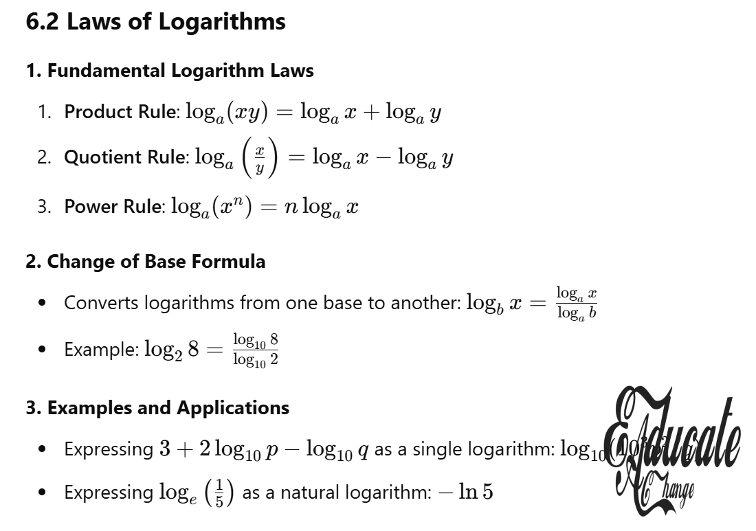
Rules of Logarithms

1. Product Rule:

• log⁡a(xy)=log⁡ax+log⁡aylog_a(xy) = log_a x + log_a y.
• Example: log⁡10(10×100)=log⁡1010+log⁡10100=1+2=3log_{10}(10 times 100) = log_{10}10 + log_{10}100 = 1 + 2 = 3.

2. Quotient Rule:

• log⁡a(xy)=log⁡ax−log⁡aylog_aleft(frac{x}{y}right) = log_a x – log_a y.
• Example: log⁡10(100010)=log⁡101000−log⁡1010=3−1=2log_{10}left(frac{1000}{10}right) = log_{10}1000 – log_{10}10 = 3 – 1 = 2.

3. Power Rule:

• log⁡a(xb)=blog⁡axlog_a(x^b) = blog_a x.
• Example: log⁡10(103)=3log⁡1010=3log_{10}(10^3) = 3log_{10}10 = 3.

4. Change of Base Rule:

• log⁡ab=log⁡cblog⁡calog_a b = frac{log_c b}{log_c a}.
• Example: Convert log⁡28log_2 8 to base 10: log⁡28=log⁡108log⁡102log_2 8 = frac{log_{10}8}{log_{10}2}.

---

Special Properties

1. Logarithm of Reciprocal:
   • log⁡a(1x)=−log⁡axlog_aleft(frac{1}{x}right) = -log_a x.
   • Example: log⁡10(0.1)=−1log_{10}(0.1) = -1, since 0.1=10−10.1 = 10^{-1}.
2. Logarithm of One:
   • log⁡a1=0log_a 1 = 0, since a0=1a^0 = 1.
3. Logarithm of the Base:
   • log⁡aa=1log_a a = 1.

---

Advanced Calculations

1. Solving Logarithmic Equations:
   • Given log⁡10x+log⁡104=log⁡1020log_{10}x + log_{10}4 = log_{10}20:
     Step 1: Apply product rule: log⁡10(4x)=log⁡1020log_{10}(4x) = log_{10}20.
     Step 2: Exponential form: 4x=204x = 20.
     Step 3: Solve x=5x = 5.
2. Finding Unknowns:
   • If 10x=50010^x = 500:
     x=log⁡10500≈2.698x = log_{10}500 approx 2.698.

---

Graphical Representation

1. Graph of y=log⁡10xy = log_{10}x:
   • The curve is defined only for x>0x > 0.
   • Passes through (1,0)(1, 0) since log⁡101=0log_{10}1 = 0.
   • Increases slowly as xx increases.
2. Comparative Behavior:
   • y=10xy = 10^x grows exponentially.
   • y=log⁡10xy = log_{10}x increases logarithmically, showing inverse behavior.

---

Applications

1. Scientific Notation:
   • Used in expressing large or small numbers.
   • Example: log⁡102.5×106≈log⁡102.5+6log_{10}2.5 times 10^6 approx log_{10}2.5 + 6.
2. Sound Intensity (Decibels):
   • Intensity II is proportional to log⁡10log_{10} of the power.
3. pH Calculations:
   • pH=−log⁡10[H+]text{pH} = -log_{10}[H^+].

---

Exercises

Practice Problems:

1. Convert 10x=10010^x = 100 into logarithmic form.
2. Solve log⁡10(x+1)=2log_{10}(x + 1) = 2 for xx.
3. Simplify log⁡1050+log⁡102log_{10}50 + log_{10}2.

Solutions:

1. x=log⁡10100=2x = log_{10}100 = 2.
2. x+1=102x + 1 = 10^2, x=99x = 99.
3. log⁡10100=2log_{10}100 = 2.

Introduction to the Laws of Logarithms

• Logarithms simplify expressions involving multiplication, division, and powers by converting operations into addition, subtraction, and multiplication, respectively.
• These laws are foundational in algebra and calculus, enabling problem-solving in exponential and logarithmic equations.

---

Key Laws of Logarithms

1. Product Law

• Definition: log⁡a(xy)=log⁡ax+log⁡aylog_a(xy) = log_a x + log_a y
• Explains that the logarithm of a product equals the sum of the logarithms of the factors.
• Example: log⁡10(8×2)=log⁡108+log⁡102log_{10}(8 times 2) = log_{10}8 + log_{10}2

  log_10(8 * 2) = log_10(8) + log_10(2)
  log_10(16) = log_10(8) + log_10(2)
  

2. Quotient Law

• Definition: log⁡a(xy)=log⁡ax−log⁡aylog_aleft(frac{x}{y}right) = log_a x – log_a y
• States that the logarithm of a quotient is the difference of the logarithms of the numerator and denominator.
• Example: log⁡10(162)=log⁡1016−log⁡102log_{10}left(frac{16}{2}right) = log_{10}16 – log_{10}2

  log_10(16 / 2) = log_10(16) - log_10(2)
  log_10(8) = 4 - 1
  

3. Power Law

• Definition: log⁡a(xn)=nlog⁡axlog_a(x^n) = nlog_a x
• Demonstrates that the logarithm of a number raised to a power equals the power times the logarithm of the base number.
• Example: log⁡10(43)=3log⁡104log_{10}(4^3) = 3log_{10}4

  log_10(4^3) = 3 * log_10(4)
  log_10(64) = 3 * log_10(4)
  

4. Change of Base Rule

• Definition: log⁡ab=log⁡cblog⁡calog_a b = frac{log_c b}{log_c a}
• Allows logarithms to be converted to a different base.
• Example: Convert log⁡28log_2 8 to base 10: log⁡28=log⁡108log⁡102log_2 8 = frac{log_{10}8}{log_{10}2}

  log_2(8) = log_10(8) / log_10(2)
  

---

Additional Properties

1. Logarithm of Reciprocal:
   • log⁡a(1x)=−log⁡axlog_aleft(frac{1}{x}right) = -log_a x
   • Example: log⁡10(0.1)=−log⁡10(10)log_{10}(0.1) = -log_{10}(10)

     log_10(1 / 10) = -log_10(10)
     

2. Logarithm of 1:
   • log⁡a1=0log_a 1 = 0, because a0=1a^0 = 1.
3. Logarithm of the Base:
   • log⁡aa=1log_a a = 1, because a1=aa^1 = a.

---

Worked Examples

Example 1: Simplify log⁡2(32)log_2(32)

• Step 1: Recognize 32=2532 = 2^5.
• Step 2: Apply the Power Law: log⁡2(25)=5log⁡2(2)log_2(2^5) = 5log_2(2).
• Step 3: Simplify: 5×1=55 times 1 = 5.

Example 2: Combine 2log⁡3(x)+log⁡3(y)2log_3(x) + log_3(y)

• Step 1: Use Power Law on 2log⁡3(x)2log_3(x): log⁡3(x2)+log⁡3(y)log_3(x^2) + log_3(y).
• Step 2: Apply Product Law: log⁡3(x2y)log_3(x^2y).

Example 3: Solve log⁡10(x)+log⁡10(x−2)=log⁡10(15)log_{10}(x) + log_{10}(x-2) = log_{10}(15)

• Step 1: Use Product Law: log⁡10[x(x−2)]=log⁡10(15)log_{10}[x(x-2)] = log_{10}(15).
• Step 2: Convert to Exponential Form: x(x−2)=15x(x-2) = 15.
• Step 3: Expand: x2−2x−15=0x^2 – 2x – 15 = 0.
• Step 4: Factorize: (x−5)(x+3)=0(x-5)(x+3) = 0.
• Step 5: Solve: x=5x = 5 (valid as x>0x > 0).

---

Graphical Representation

1. Behavior of Logarithmic Functions:
   • For y=log⁡10(x)y = log_{10}(x), the graph is only defined for x>0x > 0.
   • Passes through (1,0)(1, 0) since log⁡10(1)=0log_{10}(1) = 0.
   • Increases gradually as xx increases.
2. Reflection and Inverse:
   • Logarithmic functions are the inverse of exponential functions.
   • The graph of y=log⁡a(x)y = log_a(x) is a reflection of y=axy = a^x about y=xy = x.

---

Applications

1. Scientific Calculations:
   • Logarithms simplify operations with large or small numbers, such as in pH calculations pH=−log⁡10[H+]text{pH} = -log_{10}[H^+].
2. Sound Measurement:
   • Decibels use log⁡10log_{10}: dB=10log⁡10(II0)text{dB} = 10log_{10}left(frac{I}{I_0}right).
3. Growth and Decay:
   • Natural growth processes often involve logarithms to describe rates over time.

---

Practice Problems

1. Simplify log⁡3(27)+log⁡3(1/3)log_3(27) + log_3(1/3).
   • Solution: log⁡3(27)=3log_3(27) = 3, log⁡3(1/3)=−1log_3(1/3) = -1, so 3+(−1)=23 + (-1) = 2.
2. Express log⁡2(64)−2log⁡2(4)log_2(64) – 2log_2(4) as a single logarithm.
   • Solution: log⁡2(64)=6log_2(64) = 6, 2log⁡2(4)=42log_2(4) = 4, so log⁡2(16)=4log_2(16) = 4.
3. Solve log⁡5(x)+log⁡5(2)=1log_5(x) + log_5(2) = 1.
   • Solution: Use Product Law: log⁡5(2x)=1log_5(2x) = 1, convert: 2x=52x = 5, x=52x = frac{5}{2}.

Introduction to Solving Logarithmic Equations

• Logarithmic equations are those that include logarithms of variables.
• To solve such equations:
  • Use the laws of logarithms to simplify expressions.
  • Convert between logarithmic and exponential forms when needed.
  • Check the solution for validity, as logarithms are undefined for non-positive arguments.

---

Types of Logarithmic Equations

1. Single Logarithmic Term:
   • Example: log⁡10x=2log_{10}x = 2.
   • Solution:
     • Convert to exponential form: 102=x10^2 = x.
     • Result: x=100x = 100.
2. Equations with Multiple Logarithms:
   • Combine terms using the laws of logarithms.

---

Procedure for Solving

1. Simplify Using Logarithmic Laws:
   • Product Rule: log⁡a(xy)=log⁡ax+log⁡aylog_a(xy) = log_a x + log_a y.
   • Quotient Rule: log⁡a(xy)=log⁡ax−log⁡aylog_aleft(frac{x}{y}right) = log_a x – log_a y.
   • Power Rule: log⁡a(xn)=nlog⁡axlog_a(x^n) = nlog_a x.
2. Rewrite in Exponential Form:
   • Convert logarithms into an exponential equation when possible.
3. Solve Algebraically:
   • After simplification, solve for the variable.
4. Check Solutions:
   • Substitute back into the original equation to ensure the solution is valid.

---

Key Examples and Solutions

Example 1: Single Logarithmic Equation

Solve log⁡10x=3log_{10}x = 3.

• Step 1: Convert to exponential form: x=103x = 10^3
• Solution: x=1000x = 1000

Example 2: Equations with Addition

Solve log⁡3x+log⁡3(x−2)=1log_3x + log_3(x – 2) = 1.

• Step 1: Use the product rule:log⁡3[x(x−2)]=1log_3[x(x-2)] = 1
• Step 2: Convert to exponential form:x(x−2)=31x(x-2) = 3^1
• Step 3: Expand and solve:x2−2x−3=0x^2 – 2x – 3 = 0Factorize:

  (x−3)(x+1)=0(x – 3)(x + 1) = 0Solutions: x=3x = 3, x=−1x = -1.

• Step 4: Check for validity:
  • x=3x = 3 is valid.
  • x=−1x = -1 is invalid (logarithms undefined for x≤0x leq 0).
• Final Solution:x=3x = 3

Example 3: Equations with Subtraction

Solve log⁡2(8x)−log⁡2x=3log_2(8x) – log_2x = 3.

• Step 1: Use the quotient rule: log⁡2(8xx)=3log_2left(frac{8x}{x}right) = 3 Simplify: log⁡2(8)=3log_2(8) = 3
• Step 2: Convert to exponential form: 8=238 = 2^3
• Solution: x=1x = 1

---

Advanced Examples

Example 4: Quadratic Logarithmic Equation

Solve (log⁡2x)2−5log⁡2x+6=0(log_2x)^2 – 5log_2x + 6 = 0.

• Step 1: Substitute y=log⁡2xy = log_2x, so the equation becomes: y2−5y+6=0y^2 – 5y + 6 = 0
• Step 2: Factorize: (y−3)(y−2)=0(y – 3)(y – 2) = 0 Solutions: y=3y = 3, y=2y = 2.
• Step 3: Back-substitute: log⁡2x=3andlog⁡2x=2log_2x = 3 quad text{and} quad log_2x = 2 Convert to exponential form: x=23andx=22x = 2^3 quad text{and} quad x = 2^2
• Solution: x=8, x=4x = 8, , x = 4

---

General Tips

1. Combine Logs First:
   • Simplify multiple logarithmic terms using the laws of logarithms.
   • Example: log⁡ax+log⁡ay=log⁡a(xy)log_a x + log_a y = log_a(xy).
2. Convert Carefully:
   • When converting logarithmic equations to exponential, maintain accuracy with base and powers.
3. Exclude Invalid Solutions:
   • Logarithmic arguments must always be positive.

---

Practice Problems

1. Solve log⁡4(x−1)+log⁡4(x−3)=2log_4(x – 1) + log_4(x – 3) = 2.
   • Hint: Combine logs, then convert to exponential form.
2. Solve 3log⁡2x−log⁡2(4x)=13log_2x – log_2(4x) = 1.
   • Hint: Simplify using power and quotient rules.
3. Solve log⁡5(x+1)−log⁡5(x−1)=2log_5(x + 1) – log_5(x – 1) = 2.
   • Hint: Combine logs, then use exponential form.
4. Solve (log⁡3x)2−4log⁡3x+3=0(log_3x)^2 – 4log_3x + 3 = 0.
   • Hint: Substitute y=log⁡3xy = log_3x.

---

Summary

• Logarithmic equations can be simplified and solved using the laws of logarithms and careful algebraic manipulation.
• Always validate solutions within the domain of the logarithmic function.
• With practice, solving these equations becomes intuitive and systematic.

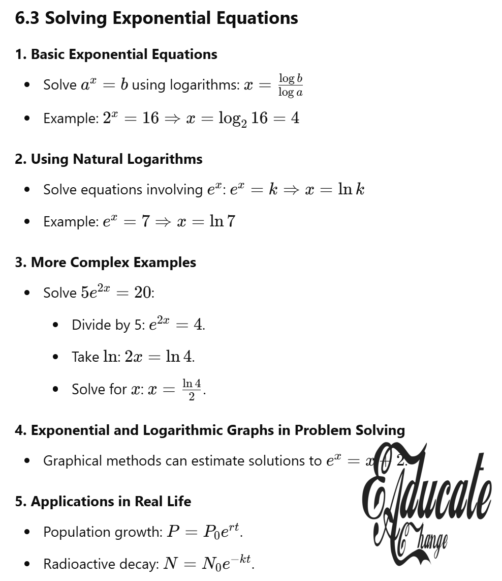
Overview of Exponential Equations

• Exponential equations contain terms where variables appear as exponents.
• Solving such equations involves:
  • Simplifying expressions.
  • Using logarithms (when the base cannot be converted to match).
  • Applying properties of exponential and logarithmic functions.
• Exponential equations are foundational in mathematics for modeling real-life phenomena such as population growth, radioactive decay, and compound interest.

---

General Steps for Solving

1. Express Terms in the Same Base:
   • If possible, rewrite both sides of the equation using the same base.

   Example: Solve 32x=273^{2x} = 27.
   Solution:

   3^{2x} = 3^3
   2x = 3
   x = frac{3}{2}
   

2. Use Logarithms for Different Bases:
   • When terms cannot be expressed in the same base, take logarithms on both sides.
   • Apply the power rule: log⁡a(bn)=nlog⁡ablog_a(b^n) = nlog_a b.

   Example: Solve 3x=403^x = 40.
   Solution:

   Take log base 10: log_{10}(3^x) = log_{10}(40)
   Use the power rule: x log_{10}(3) = log_{10}(40)
   x = frac{log_{10}(40)}{log_{10}(3)}
   

3. Isolate the Exponential Term:
   • Rearrange the equation to isolate the term with the variable exponent.
4. Check Solutions:
   • Verify that solutions satisfy the original equation and fall within its domain.

---

Key Properties of Exponential Functions

1. One-to-One Property:
   • If ax=aya^x = a^y, then x=yx = y for a>0a > 0 and a≠1a neq 1.
2. Domain and Range:
   • Exponential functions f(x)=axf(x) = a^x are defined for all xx (domain: Rmathbb{R}).
   • The range is (0,∞)(0, infty).

---

Worked Examples

Example 1: Basic Exponential Equation

Solve 2x=322^x = 32.

• Step 1: Express 32 as a power of 2: 32=2532 = 2^5
• Step 2: Rewrite the equation: 2x=252^x = 2^5
• Step 3: Equate exponents: x=5x = 5

Example 2: Using Logarithms

Solve 52x+1=2005^{2x+1} = 200.

• Step 1: Take logarithms on both sides:

  log_{10}(5^{2x+1}) = log_{10}(200)
  

• Step 2: Apply the power rule:

  (2x + 1) log_{10}(5) = log_{10}(200)
  

• Step 3: Simplify:

  2x + 1 = frac{log_{10}(200)}{log_{10}(5)}
  

• Step 4: Solve for xx:

  2x = frac{log_{10}(200)}{log_{10}(5)} - 1
  x = frac{frac{log_{10}(200)}{log_{10}(5)} - 1}{2}
  

Example 3: Quadratic in Exponents

Solve 32x−3x−6=03^{2x} – 3^x – 6 = 0.

• Step 1: Substitute y=3xy = 3^x:

  y^2 - y - 6 = 0
  

• Step 2: Factorize:

  (y - 3)(y + 2) = 0
  

• Step 3: Solve for yy:

  y = 3 quad text{(valid)} quad text{and} quad y = -2 quad text{(invalid as ( y > 0 ))}.
  

• Step 4: Back-substitute y=3xy = 3^x:

  3^x = 3 quad Rightarrow quad x = 1
  

• Solution: x=1x = 1.

Example 4: Mixed Terms

Solve 2x+1+2x=122^{x+1} + 2^x = 12.

• Step 1: Factorize 2x+12^{x+1}:

  2^{x+1} = 2 cdot 2^x
  

• Step 2: Rewrite the equation:

  2(2^x) + 2^x = 12
  

• Step 3: Simplify:

  3 cdot 2^x = 12
  

• Step 4: Solve for 2×2^x:

  2^x = 4 quad Rightarrow quad x = 2
  

---

Complex Exponential Equations

Example 5: Equations with Natural Exponents

Solve e2x−5ex+6=0e^{2x} – 5e^x + 6 = 0.

• Step 1: Substitute y=exy = e^x:

  y^2 - 5y + 6 = 0
  

• Step 2: Factorize:

  (y - 3)(y - 2) = 0
  

• Step 3: Solve for yy:

  y = 3 quad text{and} quad y = 2
  

• Step 4: Back-substitute y=exy = e^x:

  e^x = 3 quad Rightarrow quad x = ln(3)
  e^x = 2 quad Rightarrow quad x = ln(2)
  

• Solution:

  x = ln(3), ln(2)
  

Example 6: Nonlinear Forms

Solve 4x+2−4x+1=484^{x+2} – 4^{x+1} = 48.

• Step 1: Factorize 4x+24^{x+2}:

  4^{x+2} = 4^2 cdot 4^x
  

• Step 2: Rewrite the equation:

  16 cdot 4^x - 4 cdot 4^x = 48
  

• Step 3: Simplify:

  12 cdot 4^x = 48
  

• Step 4: Solve for 4×4^x:

  4^x = 4 quad Rightarrow quad x = 1
  

---

Applications of Exponential Equations

1. Growth and Decay:
   • Exponential equations describe processes like population growth (N=N0ektN = N_0 e^{kt}) and radioactive decay (N=N0e−ktN = N_0 e^{-kt}).
2. Finance:
   • Compound interest formulas involve exponential equations: A=P(1+r/n)ntA = P(1 + r/n)^{nt}.
3. Physics:
   • Half-life and decay processes use T=T0e−ktT = T_0 e^{-kt}.

---

Practice Problems

1. Solve 2x+3=642^{x+3} = 64.
2. Solve 52x+1=1255^{2x+1} = 125.
3. Solve e3x+2ex=0e^{3x} + 2e^{x} = 0.
4. Solve 3x+1+3x=363^{x+1} + 3^x = 36.

Introduction to Change of Base

• Logarithms can be rewritten in terms of a different base to make calculations easier, especially when solving logarithmic equations or when using calculators that only support certain bases (e.g., base 10 or natural logarithms).
• The Change of Base Rule provides a formula to express logarithms with one base in terms of another.

---

Change of Base Rule

Definition:

For a,b,c>0a, b, c > 0 and b,c≠1b, c neq 1,

log⁡ab=log⁡cblog⁡calog_a b = frac{log_c b}{log_c a}

Proof:

1. Let x=log⁡abx = log_a b. By definition, ax=ba^x = b.
2. Take the logarithm (base cc) of both sides: log⁡c(ax)=log⁡cblog_c(a^x) = log_c b
3. Apply the Power Rule of logarithms: x⋅log⁡ca=log⁡cbx cdot log_c a = log_c b
4. Solve for xx: x=log⁡cblog⁡cax = frac{log_c b}{log_c a}

This formula allows conversions between different logarithmic bases and is crucial when working with bases unsupported by calculators.

---

Special Cases

Base 10 (Common Logarithms):

When c=10c = 10,

log⁡ab=log⁡10blog⁡10alog_a b = frac{log_{10} b}{log_{10} a}

Natural Logarithms (Base ee):

When c=ec = e,

log⁡ab=ln⁡bln⁡alog_a b = frac{ln b}{ln a}

---

Applications of the Change of Base Rule

1. Simplifying Logarithms:
   • log⁡37=log⁡107log⁡103log_3 7 = frac{log_{10} 7}{log_{10} 3} or ln⁡7ln⁡3frac{ln 7}{ln 3}.
2. Evaluating Logarithms Without Direct Calculator Support:
   • If a calculator only supports log⁡10log_{10}, evaluate log⁡28log_2 8 as: log⁡28=log⁡108log⁡102=3log_2 8 = frac{log_{10} 8}{log_{10} 2} = 3

---

Worked Examples

Example 1: Evaluate log⁡525log_5 25

• Apply the Change of Base Rule: log⁡525=log⁡1025log⁡105log_5 25 = frac{log_{10} 25}{log_{10} 5}
• Simplify: log⁡1025=2andlog⁡105=1log_{10} 25 = 2 quad text{and} quad log_{10} 5 = 1
• Result: log⁡525=21=2log_5 25 = frac{2}{1} = 2

Example 2: Solve log⁡3(x+6)=log⁡9xlog_3(x + 6) = log_9 x

1. Change log⁡9xlog_9 x to base 3:log⁡9x=log⁡3xlog⁡39log_9 x = frac{log_3 x}{log_3 9}Simplify log⁡39=2log_3 9 = 2:

   log⁡9x=log⁡3x2log_9 x = frac{log_3 x}{2}

2. Substitute back into the equation:log⁡3(x+6)=log⁡3x2log_3(x + 6) = frac{log_3 x}{2}
3. Multiply through by 2:2log⁡3(x+6)=log⁡3x2log_3(x + 6) = log_3 x
4. Rewrite using the Power Rule:log⁡3(x+6)2=log⁡3xlog_3(x + 6)^2 = log_3 x
5. Apply the One-to-One Property:(x+6)2=x(x + 6)^2 = x
6. Expand and solve:x2+12x+36=x⇒x2+11x+36=0x^2 + 12x + 36 = x quad Rightarrow quad x^2 + 11x + 36 = 0Factorize:

   (x+9)(x+4)=0(x + 9)(x + 4) = 0Solutions: x=−9x = -9, x=−4x = -4.

7. Check validity:
   • x=−9x = -9 and x=−4x = -4 are invalid as logarithms require positive arguments.
   • No solution.

---

Benefits of the Change of Base Rule

1. Universal Applicability:
   • Simplifies complex logarithmic calculations by converting to a manageable base.
   • Enables use of calculators for non-standard bases.
2. Flexibility in Problem-Solving:
   • Combines with logarithmic properties like the Product, Quotient, and Power Rules.

---

Graphical Interpretation

• Changing the base of a logarithm transforms the graph but retains its overall shape.
• A smaller base compresses the graph horizontally, while a larger base stretches it.

---

Practice Problems

1. Evaluate log⁡749log_7 49 using base 10 and natural logarithms.
2. Simplify log⁡4(2x)log_4(2x) using the Change of Base Rule.
3. Solve log⁡5(x+1)=2log⁡5x+1log_5(x + 1) = 2log_5 x + 1.

Introduction to Natural Logarithms

• A natural logarithm is a logarithm with base ee, where ee is an irrational number approximately equal to 2.718.
• The natural logarithm is denoted by ln⁡xln x instead of log⁡exlog_e x.
  • For example: ln⁡x=log⁡exln x = log_e x.
• Natural logarithms are widely used in mathematical modeling, science, and engineering due to their natural occurrence in growth, decay, and other exponential relationships.

---

Key Properties of the Number ee

1. ee is an irrational number that arises naturally in mathematics, particularly in continuous growth and decay.
2. exe^x and ln⁡xln x are inverse functions:
   • If y=exy = e^x, then x=ln⁡yx = ln y.
   • ln⁡(ex)=xln(e^x) = x and eln⁡x=xe^{ln x} = x for x>0x > 0.
3. The graph of y=ln⁡xy = ln x is the reflection of y=exy = e^x about the line y=xy = x.

---

Rules of Natural Logarithms

All the rules of logarithms apply to natural logarithms:

1. Product Rule:ln⁡(xy)=ln⁡x+ln⁡yln(xy) = ln x + ln y
   • Example:

     ln(3 times 5) = ln 3 + ln 5
     

2. Quotient Rule:ln⁡(xy)=ln⁡x−ln⁡ylnleft(frac{x}{y}right) = ln x – ln y
   • Example:

     lnleft(frac{10}{2}right) = ln 10 - ln 2
     

3. Power Rule:ln⁡(xa)=aln⁡xln(x^a) = a ln x
   • Example:

     ln(2^3) = 3 ln 2
     

4. Logarithm of ee:ln⁡e=1ln e = 1
5. Logarithm of 1:ln⁡1=0ln 1 = 0

---

Solving Equations Involving ee and ln⁡ln

Example 1: Basic Equation

Solve ex=7e^x = 7.

• Step 1: Take the natural logarithm of both sides: ln⁡(ex)=ln⁡7ln(e^x) = ln 7
• Step 2: Simplify using ln⁡(ex)=xln(e^x) = x: x=ln⁡7x = ln 7
• Solution:

  x = ln 7 approx 1.946
  

Example 2: Quadratic Form

Solve e2x−5ex+6=0e^{2x} – 5e^x + 6 = 0.

• Step 1: Substitute y=exy = e^x, so y2−5y+6=0y^2 – 5y + 6 = 0.
• Step 2: Factorize: (y−3)(y−2)=0(y – 3)(y – 2) = 0
• Step 3: Solve for yy: y=3ory=2y = 3 quad text{or} quad y = 2
• Step 4: Back-substitute y=exy = e^x: ex=3⇒x=ln⁡3e^x = 3 quad Rightarrow quad x = ln 3 ex=2⇒x=ln⁡2e^x = 2 quad Rightarrow quad x = ln 2
• Solution:

  x = ln 3 approx 1.099 quad text{and} quad x = ln 2 approx 0.693
  

Example 3: Exponential Growth

Solve ex+2=20e^{x+2} = 20.

• Step 1: Isolate the exponential term: ex=20e2e^x = frac{20}{e^2}
• Step 2: Take the natural logarithm: x=ln⁡(20e2)x = lnleft(frac{20}{e^2}right)
• Solution:

  x = ln(20) - 2
  

---

Applications of Natural Logarithms

1. Continuous Growth and Decay:
   • N=N0ektN = N_0 e^{kt}:
     • NN: final quantity
     • N0N_0: initial quantity
     • kk: growth/decay rate
     • tt: time
2. Half-Life:
   • For radioactive decay, the half-life TT can be calculated as: T=ln⁡2kT = frac{ln 2}{k}
3. Finance:
   • Compound interest with continuous compounding: A=PertA = Pe^{rt}
     • AA: total amount
     • PP: principal
     • rr: interest rate
     • tt: time

---

Graphical Representation

1. Graph of y=exy = e^x:
   • Passes through (0,1)(0, 1) since e0=1e^0 = 1.
   • Increases rapidly for x>0x > 0.
   • Approaches 0 as x→−∞x to -infty.
2. Graph of y=ln⁡xy = ln x:
   • Passes through (1,0)(1, 0) since ln⁡1=0ln 1 = 0.
   • Undefined for x≤0x leq 0.
   • Approaches −∞-infty as x→0+x to 0^+.

---

Practice Problems

1. Solve ln⁡(x+1)=3ln(x+1) = 3.
2. Solve e2x=16e^{2x} = 16.
3. If A=100e0.05tA = 100e^{0.05t}, find tt when A=200A = 200.
4. Evaluate ln⁡0.5ln 0.5 using a calculator.

---

Summary

• Natural logarithms provide a fundamental tool in mathematical analysis, particularly for equations involving the constant ee.
• They simplify exponential equations and model natural phenomena such as population growth, radioactive decay, and financial calculations.

Introduction to Practical Applications

• Exponential equations frequently model real-world phenomena, including:
  • Temperature changes.
  • Population growth or decay.
  • Radioactive decay.
  • Compound interest and value depreciation.
• These equations provide a mathematical framework for solving problems where growth or decay occurs at a constant proportional rate.

---

Exponential Models

1. General Form:N=N0ektN = N_0 e^{kt}
   • N0N_0: Initial quantity.
   • kk: Growth (k>0k > 0) or decay (k<0k < 0) rate.
   • tt: Time.
2. Key Characteristics:
   • Growth leads to increasing values over time.
   • Decay results in diminishing values.

---

Applications in Real Life

1. Temperature Change: Newton’s Law of Cooling

• The temperature T(t)T(t) of an object changes exponentially over time: T=T0e−kt+TenvT = T_0 e^{-kt} + T_{text{env}}
  • T0T_0: Initial temperature difference between the object and its environment.
  • TenvT_{text{env}}: Ambient temperature.
  • kk: Cooling rate constant.

Example: The temperature of a hot drink T(t)T(t) is given by:

T=75e−0.02t+20T = 75e^{-0.02t} + 20

Questions:

1. Find the temperature at t=0t = 0:

   T = 75e^0 + 20 = 75(1) + 20 = 95^circ text{C}.
   

2. Find the temperature at t=6t = 6:

   T = 75e^{-0.02(6)} + 20
   T approx 75(0.885) + 20 = 86.5^circ text{C}.
   

3. Determine tt when T=65∘CT = 65^circ text{C}:

   65 = 75e^{-0.02t} + 20
   45 = 75e^{-0.02t}
   e^{-0.02t} = 0.6
   ln(0.6) = -0.02t
   t = frac{ln(0.6)}{-0.02} approx 25.5 , text{minutes}.
   

---

2. Population Growth and Decay

• Exponential equations model population dynamics: P=P0ektP = P_0 e^{kt}

Example: A species of fish in a lake has a population:

N=500e−0.1tN = 500e^{-0.1t}

Questions:

1. Initial population:

   N(0) = 500e^0 = 500.
   

2. Population after 6 weeks:

   N(6) = 500e^{-0.1(6)} = 500e^{-0.6} approx 275.
   

3. Time for population to halve:

   250 = 500e^{-0.1t}
   0.5 = e^{-0.1t}
   ln(0.5) = -0.1t
   t = frac{ln(0.5)}{-0.1} approx 6.93 , text{weeks}.
   

---

3. Radioactive Decay

• The remaining mass MM of a radioactive substance is given by: M=M0e−ktM = M_0 e^{-kt}
  • Half-life (TT) is calculated as: T=ln⁡2kT = frac{ln 2}{k}

Example: If k=0.02 per yeark = 0.02 , text{per year}, the half-life is:

T = frac{ln 2}{0.02} approx 34.66 , text{years}.

---

4. Value Depreciation

• The value VV of an asset depreciates over time: V=V0e−ktV = V_0 e^{-kt}

Example: The value of a house VV is modeled as:

V=250,000e0.05tV = 250,000e^{0.05t}

Questions:

1. Find V0V_0 if V=350,000V = 350,000 when t=3t = 3:

   350,000 = 250,000e^{0.05(3)}
   e^{0.15} approx 1.1618
   250,000(1.1618) approx 350,000.
   

2. Determine when the value doubles:

   500,000 = 250,000e^{0.05t}
   2 = e^{0.05t}
   ln(2) = 0.05t
   t = frac{ln(2)}{0.05} approx 13.86 , text{years}.
   

---

5. Bacterial Growth

• The number of bacteria NN at time tt is given by: N=N0ektN = N_0 e^{kt}

Example: If N=100N = 100 initially, and bacteria double every minute (k=ln⁡(2)k = ln(2)):

1. After 12 minutes:

   N = 100e^{12ln(2)} = 100(2^{12}) = 409,600.
   

2. Time for N>10,000,000N > 10,000,000:

   10,000,000 = 100e^{tln(2)}
   100,000 = 2^t
   t log_{10}(2) = log_{10}(100,000)
   t approx 16.6 , text{minutes}.
   

---

Graphical Representation

1. Growth:
   • Exponential growth curves rise rapidly as t→∞t to infty.
2. Decay:
   • Exponential decay curves approach zero as t→∞t to infty.

---

Practice Problems

1. A city’s population follows P=1,000,000e0.02tP = 1,000,000e^{0.02t}. Find tt when P=1,200,000P = 1,200,000.
2. A radioactive isotope decays with k=0.05k = 0.05. Calculate the half-life.
3. The temperature of an object is T=30e−0.03t+20T = 30e^{-0.03t} + 20. Determine tt when T=25T = 25.

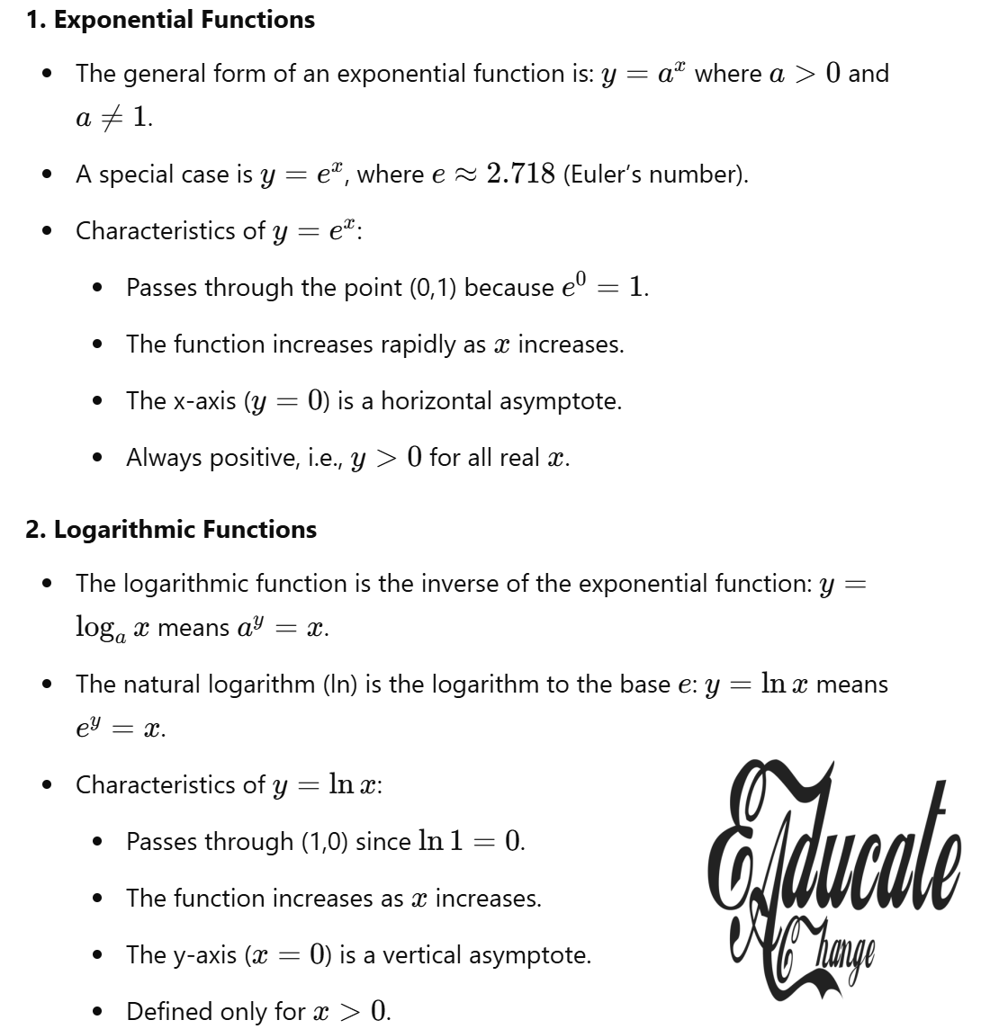
Introduction to Graphs of Exponential and Logarithmic Functions

• Exponential and logarithmic functions are foundational in mathematics, and their graphs exhibit distinct properties and behaviors.
• These functions are inversely related:
  • y=exy = e^x is the exponential function.
  • y=ln⁡xy = ln x is the natural logarithmic function.

---

Graph of y=exy = e^x

1. Key Properties:
   • y=exy = e^x intercepts the y-axis at (0,1)(0, 1).
   • For all xx, ex>0e^x > 0, ensuring y>0y > 0.
   • As x→−∞x to -infty, y→0+y to 0^+ (asymptotic to the negative x-axis).
   • As x→+∞x to +infty, y→+∞y to +infty.
2. Shape and Asymptotes:
   • The graph is increasing and smooth.
   • The curve approaches the x-axis as xx decreases but never touches it.
3. Examples:
   • At x=1x = 1, y=e1=2.718y = e^1 = 2.718.
   • At x=−1x = -1, y=e−1≈0.367y = e^{-1} approx 0.367.

---

Graph of y=ln⁡xy = ln x

1. Key Properties:
   • y=ln⁡xy = ln x intercepts the x-axis at (1,0)(1, 0).
   • The logarithmic function only exists for x>0x > 0 (undefined for x≤0x leq 0).
   • As x→0+x to 0^+, y→−∞y to -infty (asymptotic to the y-axis).
   • As x→+∞x to +infty, y→+∞y to +infty.
2. Shape and Asymptotes:
   • The graph is smooth and increasing but slows its growth as xx increases.
   • The curve approaches the y-axis as x→0x to 0, but it never touches or crosses it.
3. Examples:
   • At x=2x = 2, y=ln⁡2≈0.693y = ln 2 approx 0.693.
   • At x=0.5x = 0.5, y=ln⁡0.5≈−0.693y = ln 0.5 approx -0.693.

---

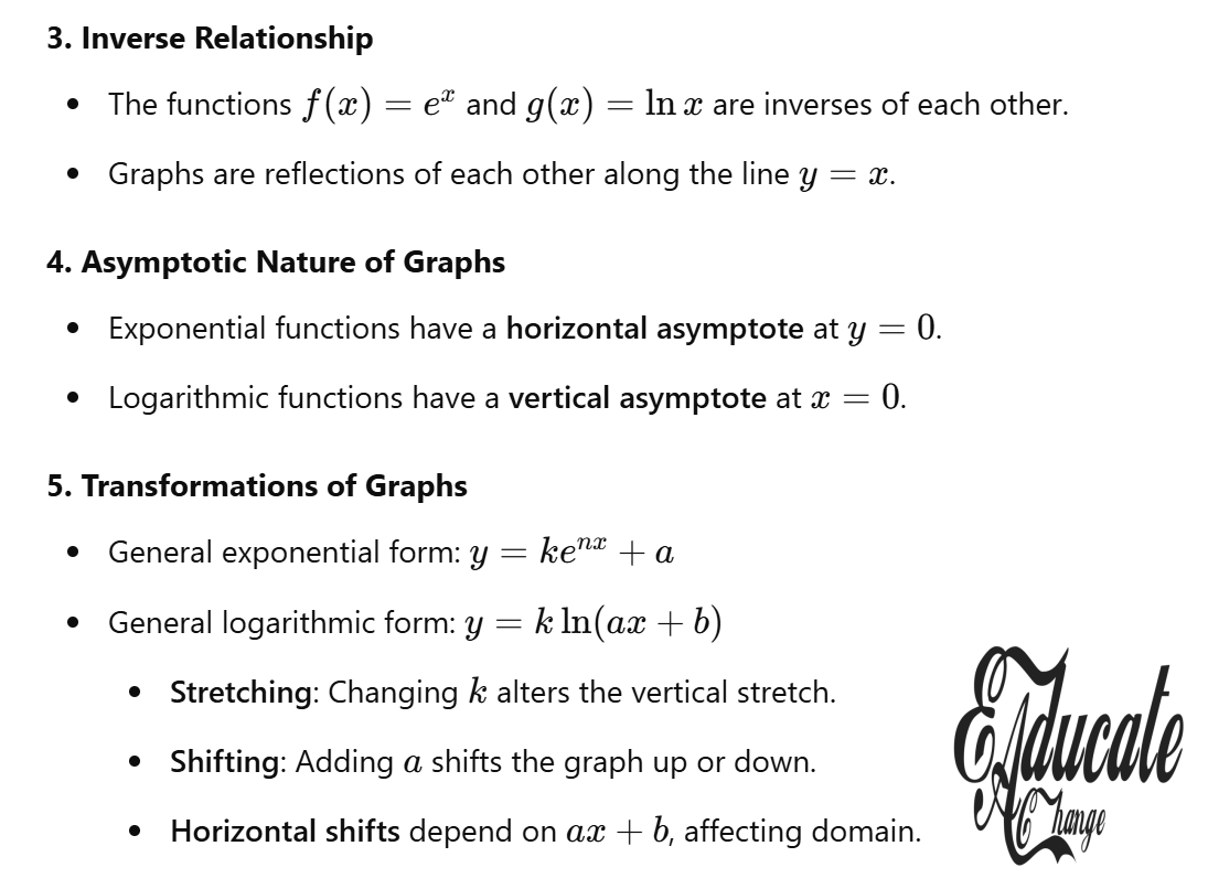
Relationship Between y=exy = e^x and y=ln⁡xy = ln x

1. Inverse Nature:
   • y=exy = e^x and y=ln⁡xy = ln x are inverse functions.
   • Their graphs are symmetric about the line y=xy = x.
2. Functional Property:
   • ln⁡(ex)=xln(e^x) = x for all xx.
   • eln⁡x=xe^{ln x} = x for x>0x > 0.

---

Transformations of Graphs

1. Exponential Functions:
   • y=kenx+ay = ke^{nx} + a:
     • kk: Stretches or compresses the graph vertically.
     • nn: Adjusts the rate of growth or decay.
     • aa: Shifts the graph vertically.

   Example:

   • y=2ex−3y = 2e^{x} – 3:
     • Intercepts the y-axis at (0,−1)(0, -1).
     • Horizontal asymptote: y=−3y = -3.
2. Logarithmic Functions:
   • y=kln⁡(ax+b)y = kln(ax + b):
     • kk: Scales the graph vertically.
     • aa, bb: Shift or compress the graph horizontally.

   Example:

   • y=4ln⁡(2x+5)y = 4ln(2x + 5):
     • Intercepts at (0,4ln⁡5)(0, 4ln 5).
     • Asymptote: x=−52x = -frac{5}{2}.

---

Worked Examples

Example 1: Sketch y=3ex−5y = 3e^{x} – 5

1. Intercepts:
   • At x=0x = 0: y=3e0−5=−2y = 3e^0 – 5 = -2.
   • As y=0y = 0: Solve 3ex−5=03e^x – 5 = 0:

     e^x = frac{5}{3}, , x = lnleft(frac{5}{3}right) approx 0.511.
     

2. Asymptotes:
   • Horizontal asymptote: y=−5y = -5.
3. Behavior:
   • As x→−∞x to -infty: y→−5y to -5.
   • As x→+∞x to +infty: y→+∞y to +infty.

---

Example 2: Sketch y=4ln⁡(2x+5)y = 4ln(2x + 5)

1. Intercepts:
   • At x=0x = 0: y=4ln⁡5≈6.44y = 4ln 5 approx 6.44.
   • As y=0y = 0: Solve ln⁡(2x+5)=0ln(2x + 5) = 0:

     2x + 5 = 1, , x = -2.
     

2. Asymptotes:
   • Vertical asymptote: x=−52x = -frac{5}{2}.
3. Behavior:
   • As x→−52+x to -frac{5}{2}^{+}: y→−∞y to -infty.
   • As x→+∞x to +infty: y→+∞y to +infty.

---

Graphical Transformations of Families

Exponential Function Families

• y=kenx+ay = ke^{nx} + a:
  • Positive kk: Growth.
  • Negative kk: Decay.
• Examples:

  For k = 1, 2, 3: Steeper growth.
  For k = -1, -2, -3: Steeper decay.
  

Logarithmic Function Families

• y=kln⁡(ax+b)y = kln(ax + b):
  • Changes in k,a,bk, a, b stretch, shift, or compress the graph.
• Examples:

  For k = 1, 2, 3: Increased vertical stretch.
  For k = -1, -2, -3: Reflection and stretch.
  

---

Practice Problems

1. Sketch y=2e−x+3y = 2e^{-x} + 3. Identify intercepts and asymptotes.
2. For y=ln⁡(x+4)−2y = ln(x + 4) – 2:
   • Find the domain.
   • Determine the x- and y-intercepts.
3. Compare the graphs of y=exy = e^x and y=ln⁡xy = ln x. Highlight symmetry.

Introduction

• Inverse Functions:
  • The inverse of a function f(x)f(x) is a function g(x)g(x) such that f(g(x))=xf(g(x)) = x and g(f(x))=xg(f(x)) = x.
  • For a function to have an inverse, it must be one-to-one.
• Logarithmic and exponential functions are inverses of each other:
  • y=exy = e^x and y=ln⁡xy = ln x are inverse functions.
  • Similarly, y=axy = a^x and y=log⁡axy = log_a x are inverses.

---

Finding the Inverse

General Steps:

1. Write the Function as y=f(x)y = f(x):
   • Example: y=2ex+3y = 2e^x + 3.
2. Interchange xx and yy:
   • Example: x=2ey+3x = 2e^y + 3.
3. Solve for yy:
   • Isolate yy to find the inverse.
4. Express yy as f−1(x)f^{-1}(x):
   • Final result represents the inverse function.

---

Worked Examples

Example 1: Inverse of an Exponential Function

Find the inverse of f(x)=2ex+3f(x) = 2e^x + 3 for x∈Rx in mathbb{R}.

• Step 1: Write the function as yy:y=2ex+3y = 2e^x + 3
• Step 2: Interchange xx and yy:x=2ey+3x = 2e^y + 3
• Step 3: Solve for yy:x−3=2eyx – 3 = 2e^y x−32=eyfrac{x – 3}{2} = e^y y=ln⁡(x−32)y = lnleft(frac{x – 3}{2}right)
• Step 4: Write the inverse:f−1(x)=ln⁡(x−32)f^{-1}(x) = lnleft(frac{x – 3}{2}right)

Example 2: Inverse of a Logarithmic Function

Find the inverse of f(x)=3ln⁡(2x−4)f(x) = 3ln(2x – 4), for x>2x > 2.

• Step 1: Write the function as yy:y=3ln⁡(2x−4)y = 3ln(2x – 4)
• Step 2: Interchange xx and yy:x=3ln⁡(2y−4)x = 3ln(2y – 4)
• Step 3: Solve for yy:x3=ln⁡(2y−4)frac{x}{3} = ln(2y – 4) ex3=2y−4e^{frac{x}{3}} = 2y – 4 2y=ex3+42y = e^{frac{x}{3}} + 4 y=ex3+42y = frac{e^{frac{x}{3}} + 4}{2}
• Step 4: Write the inverse:f−1(x)=ex3+42f^{-1}(x) = frac{e^{frac{x}{3}} + 4}{2}

---

Properties of Inverse Functions

1. Symmetry:
   • The graph of f(x)f(x) and its inverse f−1(x)f^{-1}(x) are symmetric about the line y=xy = x.
2. Domain and Range:
   • The domain of f(x)f(x) becomes the range of f−1(x)f^{-1}(x), and vice versa.
3. Exponential-Logarithmic Pair:
   • For f(x)=exf(x) = e^x, f−1(x)=ln⁡xf^{-1}(x) = ln x.
   • For f(x)=axf(x) = a^x, f−1(x)=log⁡axf^{-1}(x) = log_a x.

---

Applications

1. Exponential Growth and Decay:
   • Inverse functions help solve for time (tt) in models like N=N0ektN = N_0 e^{kt}.
   • Example:

     If N = 500e^{0.02t}, solve for t when N = 1000:
     

     t=ln⁡(2)0.02=34.66 years.‘‘‘t = frac{ln(2)}{0.02} = 34.66 , text{years.} “`

2. Logarithmic Scales:
   • Inverse functions are used to interpret logarithmic scales, such as pH (−log⁡[H+]-log[H^+]) or decibels (10log⁡(I/I0)10log(I/I_0)).
3. Finance:
   • Exponential and logarithmic inverses solve for time or interest rates in compound interest: A=Pert  ⟹  t=ln⁡(A/P)r.A = P e^{rt} quad implies quad t = frac{ln(A/P)}{r}.

---

Graphical Representations

1. Exponential Function y=exy = e^x:
   • Passes through (0,1)(0, 1).
   • Rapidly increases for x>0x > 0 and asymptotically approaches y=0y = 0 for x<0x < 0.
2. Logarithmic Function y=ln⁡xy = ln x:
   • Passes through (1,0)(1, 0).
   • Defined for x>0x > 0, with y→−∞y to -infty as x→0+x to 0^+.
3. Symmetry:
   • Both graphs are reflections of each other across y=xy = x.

---

Practice Problems

1. Find the inverse of f(x)=5e2x+4f(x) = 5e^{2x} + 4.
2. Determine the domain and range of f−1(x)f^{-1}(x) for f(x)=2ln⁡(x−1)+3f(x) = 2ln(x – 1) + 3.
3. Sketch y=exy = e^x and y=ln⁡xy = ln x, showing their symmetry about y=xy = x.